Understanding Monetary Policy Implementation

Economic Quarterly—Volume 94, Number 3—Summer 2008—Pages 235–263

Understanding Monetary

Policy Implementation

Huberto M. Ennis and Todd Keister

ver the last two decades, central banks around the world have adopted

a common approach to monetary policy that involves targeting the

value of a short-term interest rate. In the United States, for example,

the Federal Open Market Committee (FOMC) announces a rate that it wishes

to prevail in the federal funds market, where commercial banks lend balances

held at the Federal Reserve to each other overnight. Changes in this short-

term interest rate eventually translate into changes in other interest rates in the

economy and thereby inﬂuence the overall level of prices and of real economic

activity.

Once a target interest rate is announced, the problem of implementation

arises: How can a central bank ensure that the relevant market interest rate

stays at or near the chosen target? The Federal Reserve has a variety of tools

available to inﬂuence the behavior of the interest rate in the federal funds

market (called the fed funds rate). In general, the Fed aims to adjust the total

supply of reserve balances so that it equals demand at exactly the target rate

of interest. This process necessarily involves some estimation, since the Fed

does not know the exact demand for reserve balances, nor does it completely

control the supply in the market.

A critical issue in the implementation process, therefore, is the sensitivity

of the market interest rate to unanticipated changes in supply and/or demand.

Some of the material in this article resulted from our participation in the Federal Reserve

System task force created to study paying interest on reserves. We are very grateful to the

other members of this group, who patiently taught us many of the things that we discuss here.

We also would like to thank Kevin Bryan, Yash Mehra, Rafael Repullo, John Walter, John

Weinberg, and the participants at the 2008 Columbia Business School/New York Fed confer-

ence on “The Role of Money Markets” for useful comments on a previous draft. All remain-

ing errors are, of course, our own. The views expressed here do not necessarily represent

those of the Federal Reserve Bank of New York, the Federal Reserve Bank of Richmond,

or the Federal Reserve System. Ennis is on leave from the Richmond Fed at University

Carlos III of Madrid and Keister is at the Federal Reserve Bank of New York. E-mails:

[email protected], Todd.Keister@ny.frb.org.

236 Federal Reserve Bank of Richmond Economic Quarterly

If small estimation errors lead to large swings in the interest rate, a central

bank will ﬁnd it difﬁcult to effectively implement monetary policy, that is, to

consistently hit the target rate. The degree of sensitivity depends on a variety

of factors related to the design of the implementation process, such as the time

period over which banks are required to hold reserves and the interest rate, if

any, that a central bank pays on reserve balances.

The ability to hit a target interest rate consistently plays a critical role in a

central bank’s communication policy. The overall effectiveness of monetary

policy depends, in part, on individuals’ perceptions of the central bank’s ac-

tions and objectives. If the market interest rate were to deviate consistently

from the central bank’s announced target, individuals might question whether

these deviations simply represent glitches in the implementation process or

whether they instead represent an unannounced change in the stance of mon-

etary policy. Sustained deviations of the average fed funds rate from the

FOMC’s target in August 2007, for example, led some media commentators

to claim that the Fed had engaged in a “stealth easing,” taking actions that

lowered the market interest rate without announcing a change in the ofﬁcial

target.

In such times, the ability to hit a target interest rate consistently allows

the central bank to clearly (and credibly) communicate its policy to market

participants.

Under most circumstances, the Fed changes the total supply of reserve

balances available to commercial banks by exchanging government bonds

or other securities for reserves in an open market operation. Occasionally,

the Fed also provides reserves directly to certain banks through its discount

window. In some situations, the Fed has developed other, ad hoc methods

of inﬂuencing the supply and distribution of reserves in the market. For

example, during the recent period of ﬁnancial turmoil, the market’s ability to

smoothly distribute reserves across banks became partially impaired, which

led to signiﬁcant ﬂuctuations in the average fed funds rate both during the day

and across days. In December 2007, partly to address these problems, the Fed

introduced the Term Auction Facility (TAF), a bimonthly auction of a ﬁxed

quantity of reserve balances to all banks eligible to borrow at the discount

window. In principle, the TAF has increased these banks’ ability to access

reserves directly and, in this way, has helped ease the pressure on the market

to redistribute reserves and avoid abnormal ﬂuctuations in the market rate.

Such operations, of course, need to be managed so as to achieve the ultimate

goal of implementing the chosen target interest rate. Balancing the demand

and supply of reserves is at the very core of this problem.

This article presents a simple analytical framework for understanding the

process of monetary policy implementation and the factors that inﬂuence a

See, for example, “A ‘Stealth Easing’ by the Fed?” (Coy 2007).

H. M. Ennis and T. Keister: Monetary Policy Implementation 237

central bank’s ability to keep the market interest rate close to a target level.

We present this framework graphically, focusing on how various features of

the implementation process affect the sensitivity of the market interest rate to

unanticipated changes in supply or demand. We discuss the current approach

used by the Fed, including the use of reserve maintenance periods to decrease

this sensitivity. We also show how this framework can be used to study a wide

range of issues related to monetary policy implementation.

In 2006, the U.S. Congress enacted legislation that will give the Fed the

authority to pay interest on reserve balances beginning in October 2011.

We use our simple framework to illustrate how the ability to pay interest on

reserves can be a useful policy tool for a central bank. In particular, we show

how paying interest on reserves can decrease the sensitivity of the market

interest rate to estimation errors and, thus, enable a central bank to better

achieve its desired interest rate.

The model we present uses the basic approach to reserve management

introduced by Poole (1968) and subsequently advanced by many others (see,

for example, Dotsey 1991; Guthrie and Wright 2000; Bartolini, Bertola, and

Prati 2002; and Clouse and Dow 2002). The speciﬁc details of our formaliza-

tion closely follow those in Ennis and Weinberg (2007), after some additional

simpliﬁcations that allow us to conduct all of our analysis graphically. Ennis

and Weinberg (2007) focused on the interplay between daylight credit and

the Fed’s overnight treatment of bank reserves. In this article, we take a more

comprehensive view of the process of monetary policy implementation and we

investigate several important topics, such as the role of reserve maintenance

periods, which were left unexplored by Ennis and Weinberg (2007).

1. U.S. MONETARY POLICY IMPLEMENTATION

Banks hold reserve balances in accounts at the Federal Reserve in order to

satisfy reserve requirements and to be able to make interbank payments. Dur-

ing the day, banks can also access funds by obtaining an overdraft from their

reserve accounts at the Fed. The terms by which the Fed provides daylight

credit are one of the factors determining the demand for reserves by banks.

To adjust their reserve holdings, banks can borrow and lend balances in

the fed funds market, which operates weekdays from 9:30 a.m. to 6:30 p.m.

A bank wanting to decrease its reserve holdings, for example, can do so in this

market by making unsecured, overnight loans to other banks.

The fed funds market plays a crucial role in monetary policy implementa-

tion because this is where the Federal Reserve intervenes to pursue its policy

objectives. The stance of monetary policy is decided by the FOMC, which

After this article was written, the effective date for the authority to pay interest on reserves

was moved to October 1, 2008, by the Emergency Economic Stabilization Act of 2008.

238 Federal Reserve Bank of Richmond Economic Quarterly

selects a target for the overnight interest rate prevailing in this market. The

Committee then instructs the Open Market Desk to adjust, via open market

operations, the supply of reserve balances so as to steer the market interest

rate toward the selected target.

The Desk conducts open market operations largely by arranging repur-

chase agreements (repos) with primary securities dealers in a sealed-bid,

discriminatory price auction. Repos involve using reserve balances to pur-

chase securities with the explicit agreement that the transaction will be

reversed at maturity. Repos usually have overnight maturity, but the Desk

also employs other maturities (for example, two-day and two-week repos are

commonly used). Open market operations are typically conducted early in

the morning when the market for repos is most active.

The new reserves created in an open market operation are deposited in the

participating securities dealers’ bank accounts and, hence, increase the total

supply of reserves in the banking system. In this way, each day the Desk

tries to move the supply of reserve balances as close as possible to the level

that would leave the market-clearing interest rate equal to the target rate. An

essential step in this process is accurately forecasting both aggregate reserve

demand and those changes in the existing supply of reserve balances that are

due to autonomous factors beyond the Fed’s control, such as payments into

and out of the Treasury’s account and changes in the quantity of currency in

circulation. Forecasting errors will lead the actual supply of reserve balances

to deviate from the intended level and, hence, will cause the market rate to

diverge from the target rate, even if reserve demand is perfectly anticipated.

Reserve requirements in the United States are calculated as a proportion

of the quantity of transaction deposits on a bank’s balance sheet during a two-

week computation period prior to the start of the maintenance period. These

requirements can be met through a combination of vault cash and reserve

balances held at the Fed. During the two-week reserve maintenance period,

a bank’s end-of-day reserve balances must, on average, equal the reserve

requirement minus the quantity of vault cash held during the computation

period. Reserve requirements make a large portion of the demand for reserve

balances fairly predictable, which simpliﬁes monetary policy implementation.

Reserve maintenance periods allow banks to spread out their reserve hold-

ings over time without having to scramble for funds to meet a requirement at

the end of each day. However, near the end of the maintenance period, this

averaging effect tends to lose force. On the last day of the period, a bank has

some level of remaining requirement that must be met on that day. This gen-

erates a fairly inelastic demand for reserve balances and makes implementing

a target interest rate more challenging. For this reason, the Fed allows banks

See Hilton and Hrung (2007) for a more detailed overview of the Fed’s monetary policy

implementation procedures.

H. M. Ennis and T. Keister: Monetary Policy Implementation 239

holding excess or deﬁcient balances at the end of a maintenance period to carry

over those balances and use them to satisfy up to 4 percent of their requirement

in the following period.

If a bank ﬁnds itself short of reserves at the end of the maintenance period,

even after taking into account the carryover possibilities, it has several options.

It can try to ﬁnd a counterparty late in the day offering an acceptable interest

rate. However, this may not be feasible because of an aggregate shortage of

reserve balances or because of the existence of trading frictions in this market.

A second alternative is to borrow at the discount window of its corresponding

Federal Reserve Bank.

The discount window offers collateralized overnight

loans of reserves to banks that have previously pledged appropriate collateral.

Discount window loans are typically charged an interest rate that is 100 basis

points above the target fed funds rate, although changing the size of this gap

is possible and has been used, at times, as a policy instrument. Finally, if

the bank does not have the appropriate collateral or chooses not to borrow

at the discount window for other reasons, it will be charged a penalty fee

proportional to the amount of the shortage.

Currently, banks earn no interest on the reserve balances they hold in

their accounts at the Federal Reserve.

This situation may soon change: The

Financial Services Regulatory Relief Act of 2006 allows the Fed to begin

paying interest on reserve balances in October 2011. The Act also includes

provisions that give the Fed more ﬂexibility in determining reserve require-

ments, including the ability to eliminate the requirements altogether. Thus,

this legislation opens the door to potentially substantial changes in the way

the Fed implements monetary policy. To evaluate the best approach within the

new, broader set of alternatives, it seems useful to develop a simple analytical

framework that is able to address many of the relevant aspects of the problem.

We introduce and discuss such a framework in the sections that follow.

2. THE DEMAND FOR RESERVES

In this section, we present a simple framework that is useful for understanding

banks’demand for reserves. In this framework, a bank holds reserves primarily

to satisfy reserve requirements, although other factors, such as the desire to

make interbank payments, may also play a role. Since banks cannot fully

predict the timing of payments, they face uncertainty about the net outﬂows

from their reserve accounts and, therefore, are typically unable to exactly

satisfy their reserve requirements. Instead, they must balance the possibility

There are 12 regions and corresponding Reserve Banks in the Federal Reserve System. For

each commercial bank, the corresponding Reserve Bank is determined by the region where the

commercial bank is headquartered.

See footnote 2.

240 Federal Reserve Bank of Richmond Economic Quarterly

of holding excess reserve balances—and the associated opportunity cost—

against the possibility of being penalized for a reserve deﬁciency. A bank’s

demand for reserves results from optimally balancing these two concerns.

The Basic Framework

We assume banks are risk-neutral and maximize expected proﬁts. At the

beginning of the day, banks can borrow and lend reserves in a competitive

interbank market. Let R be the quantity of reserves chosen by a bank in

the interbank market. The central bank affects the supply of reserves in this

market by conducting open market operations. Total reserve supply is equal

to the quantity set by the central bank through its operations, adjusted by a

potentially random amount to reﬂect unpredictable changes in autonomous

factors.

During the day, each bank makes payments to and receives payments from

other banks. To keep things as simple as possible, suppose that each bank

will make exactly one payment and receive exactly one payment during the

“middle” part of the day. Furthermore, suppose that these two payment ﬂows

are of exactly the same size, P

> 0, and that this size is nonstochastic. How-

ever, the order in which these payments occur during the day is random; some

banks will receive the incoming payment before making the outgoing one,

while others will make the outgoing payment before receiving the incoming

one.

At the end of the day, after the interbank market has closed, each bank

experiences another payment shock, P , that affects its end-of-day reserve

balance. The value of P can be either positive, indicating a net outﬂow of

funds, or negative, indicating a net inﬂow of funds. We assume that the

payment shock, P , is uniformly distributed on the interval



−

P,P



. The

value of this shock is not yet known when the interbank market is open; hence,

a bank’s demand for reserves in this market is affected by the distribution of

the payment shock and not the realization.

We assume, as a starting point, that a bank must meet a given reserve

requirement, K, at the end of each day.

If the bank ﬁnds itself holding fewer

than K reserves at the end of the day, after the payment shock P has been

realized, it must borrow funds at a “penalty” rate of interest, r

, to satisfy the

requirement. This rate can be thought of as the rate charged by the central

bank on discount window loans, adjusted to take into account any “stigma”

associated with using this facility. In reality, a bank may pay a deﬁciency

fee instead of borrowing from the discount window or it may borrow funds

We discuss more complicated systems of reserve requirements later, including multiple-day

maintenance periods. For the logic in the derivations that follow, the particular value of K does

not matter. The case of K = 0 corresponds to a system without reserve requirements.

H. M. Ennis and T. Keister: Monetary Policy Implementation 241

in the interbank market very late in the day when this market is illiquid. In

the model, the rate r

simply represents the cost associated with a late-day

reserve deﬁciency, whatever the source of that cost may be.

The speciﬁc assumptions we make about the number and size of payments

that a bank sends are not important; they only serve to keep the analysis free

of unnecessary complications. Two basic features of the model are important.

First, the bank cannot perfectly anticipate its end-of-day reserve position.

This uncertainty creates a “precautionary” demand for reserves that smoothly

responds to changes in the interest rate. Second, a bank makes payments

during the day as a part of its normal operations and the pattern of these

payments can potentially lead to an overdraft in the bank’s reserve account.

We initially assume that the central bank offers daylight credit to banks to cover

such overdrafts at no charge. We study the case where daylight overdrafts are

costly later in this section.

The Benchmark Case

We begin by analyzing a simple benchmark case; we show later in this section

how the framework can be extended to include a variety of features that are

important in reality. In the benchmark case, banks must meet their reserve

requirement at the end of each day, and the central bank pays no interest

on reserves held by banks overnight. Furthermore, the central bank offers

daylight credit free of charge.

Figure 1 depicts an individual bank’s demand for reserves in the interbank

market under this benchmark scenario. On the horizontal axis we measure the

bank’s choice of reserve holdings before the late-day payment is realized.On

the vertical axis we measure the market interest rate for overnight loans. To

draw the demand curve, we ask: Given a particular value for the interest rate,

what quantity of reserves would the bank demand to hold if that rate prevailed

in the market?

A bank would be unwilling to hold any reserves if the market interest rate

were higher than r

. If the market rate were higher than the penalty rate,

the bank would choose to meet its requirement entirely by borrowing from

the discount window. It would actually like to borrow even more than its

requirement and lend the rest out at the higher market rate, but this fact is not

important for the analysis. The important point is simply that there will be no

demand for (nonborrowed) reserves for any interest rate larger than r

When the market interest rate exactly equals the penalty rate, r

, a bank

would be indifferent between holding any amount of reserves between zero

and K −

P and, hence, the demand curve is horizontal at r

. As long as

the bank’s reserve holdings, R, are smaller than K −

P , the bank will need

to borrow at the discount window to satisfy its reserve requirement, K,even

if the late-day inﬂow of funds into the bank’s reserve account is the largest

242 Federal Reserve Bank of Richmond Economic Quarterly

Figure 1 Benchmark Demand for Reserves

K-P

K+P

Demand for

Reserves

possible value, P .

The alternative would be to borrow more reserves in the

market to reduce this potential need for discount window lending. Since the

market rate is equal to the penalty rate, both strategies deliver the same level

of proﬁt and the bank is indifferent between them.

For market interest rates below the penalty rate, however, a bank will

choose to hold at least K −

P reserves. As discussed above, if the bank held

fewer than K −

P reserves it would be certain to need to borrow from the

discount window, which would not be an optimal choice when the market

rate is lower than the discount rate. The bank’s demand for reserves in this

situation can be described as “precautionary” in the sense that the bank chooses

its reserve holdings to balance the possibility of falling short of the requirement

against the possibility of ending up with extra reserves in its account at the

end of the day.

To see this, note that even in the best case scenario the bank will ﬁnd itself holding R +P

reserves after the arrival of the late-day payment ﬂow. When R<K−

P , the bank’s end-of-day

holdings of reserves is insufﬁcient to satisfy its reserve requirement, K, unless it takes a loan at

the discount window.

H. M. Ennis and T. Keister: Monetary Policy Implementation 243

If the market interest rate were very low—close to zero—the opportunity

cost of holding reserves would be very small. In this case, the bank would

hold enough precautionary reserves so that it is virtually certain that unfore-

seen movements on its balance sheet will not decrease its reserves below the

required level. In other words, the bank will hold K +

P reserves in this

case. If the market interest rate were exactly zero, there would be no oppor-

tunity cost of holding reserves. The demand curve is, therefore, ﬂat along the

horizontal axis after K +

P .

In between the two extremes, K −

P and K + P , the demand for reserves

will vary inversely with the market interest rate measured on the vertical axis;

this portion of the demand curve is represented by the downward-sloping

line in Figure 1. The curve is downward-sloping for two reasons. First,

the market interest rate represents the opportunity cost of holding reserves

overnight. When this rate is lower, ﬁnding itself with excess balances is less

costly for the bank and, hence, the bank is more willing to hold precautionary

balances. Second, when the market rate is lower, the relative cost of having to

access the discount window is larger, which also tends to increase the bank’s

precautionary demand for reserves.

The linearity of the downward-sloping part of the demand curve results

from the assumption that the late-day payment shock is uniformly distributed.

With other probability distributions, the demand curve will be nonlinear, but

its basic shape will remain unchanged. In particular, the points where the

demand curve intersects the penalty rate, r

, and the horizontal axis will be

the same for any distribution with support



−

P,P



The Equilibrium Interest Rate

Suppose, for the moment, that there is a single bank in the economy. Then

the demand curve in Figure 1 also represents the total demand for reserves.

Let S denote the total supply of reserves in the interbank market, as jointly

determined by the central bank’s open market operations and autonomous

factors. Then the equilibrium interest rate is determined by the height of the

demand curve at point S. As shown in the diagram, there is a unique level of

reserve supply, S

, that will generate a given target interest rate, r

Now suppose there are many banks in the economy, but they are all identi-

cal in that they have the same level of required reserves, face the same payment

shock, etc. When there are many banks, the total demand for reserves can be

found by simply “adding up” the individual demand curves. For any interest

The support of the probability distribution is the set of values of the payment shock that

is assigned positive probability. An explicit formula for the demand curve in the uniform case is

derived in Ennis and Weinberg (2007). If the shock instead had an unbounded distribution, such

as the normal distribution used by Whitesell (2006) and others, the demand curve would asymptote

to the penalty rate and the horizontal axis but never intersect them.

244 Federal Reserve Bank of Richmond Economic Quarterly

rate r, total demand is simply the sum of the quantity of reserves demanded

by each individual bank.

For presentation purposes, it is useful to look at the average demand for

reserves, that is, the total demand divided by the number of banks. When

all banks are identical, the average demand is exactly equal to the demand

of each individual bank. In other words, in the benchmark case where banks

are identical, the demand curve in Figure 1 also represents the aggregate

demand for reserves, expressed in per-bank terms. The determination of the

equilibrium interest rate then proceeds exactly as in the single-bank case. In

particular, the market-clearing interest rate will be equal to the target rate, r

if and only if reserve supply (expressed in per-bank terms) is equal to S

Note that the central bank has two distinct ways in which it can potentially

affect the market interest rate: changing the supply of reserves available in the

market and changing (either directly or indirectly) the penalty rate. Suppose,

for example, that the central bank wishes to decrease the market interest rate.

It could either increase the supply of reserves through open market operations,

leading to a movement down the demand curve, or it could decrease the penalty

rate, which would rotate the demand curve downward while leaving the supply

of reserves unchanged. Both policies would cause the market interest rate

to fall.

Heterogeneity

While the assumption that all banks are identical was useful for simplifying

the presentation above, it is clearly a poor representation of reality in most

economies. The United States, for example, has thousands of banks and other

depository institutions that differ dramatically in size, range of activities, etc.

We now show how the analysis above changes when there is heterogeneity

among banks and, in particular, how the size distribution of banks might affect

the aggregate demand for reserves.

Each bank still has a demand curve of the form depicted in Figure 1, but

now these curves can be different from each other because banks may have

different levels of required reserves, face different distributions of the payment

shock, and/or face different penalty rates. These individual demand curves

can be aggregated exactly as before: For any interest rate r, the total demand

for reserves is simply the sum of the quantity of reserves demanded by each

individual bank. The aggregate demand curve, expressed in per-bank terms,

will again be similar to that presented in Figure 1, with the exact shape being

determined by the properties of the various individual demands. If different

banks have different levels of required reserves, for example, the requirement

K in the aggregate demand curve will be equal to the average of the individual

banks’ requirements.

H. M. Ennis and T. Keister: Monetary Policy Implementation 245

Our interest here is in studying how bank heterogeneity affects the prop-

erties of this demand curve. We focus on heterogeneity in bank size, which

is particularly relevant in the United States, where there are some very large

banks and thousands of smaller banks. We ask how large banks may differ

from small banks in the context of the simple framework and how the pres-

ence of both large and small banks might affect the properties of the aggregate

demand curve. To simplify the presentation, we study the three possible

dimensions of heterogeneity addressed by the model one at a time. In reality,

of course, the three cases are closely intertwined.

Size of Requirements

Perhaps the most natural way of capturing differences in bank size is by

allowing for heterogeneity in reserve requirements. When requirements are

calculated as a percentage of the deposit base, larger banks will tend to have a

larger level of required reserves in absolute terms. Suppose, then, that banks

have different levels of K, but they face the same late-day payment shock and

the same penalty rate for a reserve deﬁciency. How would the size distribution

of banks affect the aggregate demand for reserves in this case?

To begin, note that in Figure 1 the slope of the demand curve is independent

of the size of the bank’s reserve requirement, K. To see why this is the case,

consider an increase in the value of K. Since both K −

P and K + P become

larger numbers, the demand curve in Figure 1 shifts to the right. Notice

that these two points shift exactly the same distance, leaving the slope of the

downward-sloping segment of the demand curve unchanged.

Simple aggregation then shows that the slope of the aggregate demand

curve will be independent of the size distribution of banks. In other words, for

the case of heterogeneity in K, the sensitivity of reserve demand to changes in

the interest rate does not depend at all on whether the economy is comprised

of only large banks or, as in the United States, has a few large banks and very

many small ones.

Adding heterogeneity in reserve requirements does generate an interesting

implication for the distribution of excess reserve holdings across banks. If

large and small banks face similar (effective) penalty rates and are not too

different in their exposure to late-day payment uncertainty, then the framework

suggests that all banks should hold similar quantities of precautionary reserves.

In other words, for a given level of the interest rate, the difference between

the chosen reserve balances, R, and the requirement, K, should be similar for

all banks. After the payment shocks are realized, of course, some banks will

end up holding excess reserves and others will end up needing to borrow. On

average, however, a large bank and a small one should ﬁnish the period with

comparable levels of excess reserves. If the banking system is composed of

a relatively small number of large banks and a much larger number of small

246 Federal Reserve Bank of Richmond Economic Quarterly

Figure 2 Heterogeneity

Small Banks

Large Banks

Panel A

Panel B

Low-Variance

Demand

High-Variance

Demand

K+P

K-P K-P

K+P K+P

banks, then the majority of the excess reserves in the banking system will be

held by small banks, simply because there are so many more of them. Even if

large banks hold the majority of total reserve balances because of their larger

requirements, most of the excess reserve balances will be held by small banks.

This implication is broadly in line with the data for the United States.

The Penalty Rate

Another way in which small banks might differ from large ones is the penalty

rate they face if they need to borrow to avoid a reserve deﬁciency. To be

H. M. Ennis and T. Keister: Monetary Policy Implementation 247

eligible to borrow at the discount window, for example, a bank must establish

an agreement with its Reserve Bank and post collateral. This ﬁxed cost may

lead some smaller banks to forgo accessing the discount window and instead

borrow at a very high rate in the market (or pay the reserve deﬁciency fee)

when necessary. Smaller banks may also have fewer established relationships

with counterparties in the fed funds market and, as a consequence, may ﬁnd it

more difﬁcult to borrow at a favorable interest rate late in the day (see Ashcraft,

McAndrews, and Skeie 2007).

Suppose small banks do face a higher penalty rate, such as the value r

depicted in Figure 2, Panel A, while larger banks face a lower rate, r

. The

ﬁgure is drawn as if the two banks have the same level of requirements, but

this is done only to make the comparison between the curves clear. The ﬁgure

shows two immediate implications of this type of heterogeneity. First, at

any given interest rate, small banks will hold a higher level of precautionary

reserves, that is, they will choose a larger reserve balance relative to their

level of required reserves. In the ﬁgure, the smaller bank will hold a quantity

while the larger bank holds only S

, even though—in this example—both

face the same requirement and the same uncertainty about their end-of-day

balance. As a result, the distribution of excess reserves in the economy will

tend to be skewed even more heavily toward small banks than the earlier

discussion would suggest.

The second implication shown in Figure 2, Panel A is that the demand

curve for small banks has a steeper slope. In an economy with a large number

of small banks, therefore, the aggregate demand curve will tend to be steeper,

meaning that average reserve balances will be less sensitive to changes in the

market interest rate. Notice that this result obtains even though there are no

costs of reserve management in the model.

Support of the Payment Shock

A third way in which banks potentially differ from each other is in the distri-

bution of the late-day payment shock they face. Figure 2, Panel B depicts two

demand curves, one for a bank facing a higher variance of this distribution and

one for a bank facing a lower variance. The ﬁgure shows that having more

uncertainty about the end-of-day reserve position leads to a ﬂatter demand

curve and, hence, a reserve balance that is more responsive to changes in the

interest rate.

In this case, it is not completely clear which curve corresponds better to

large banks and which to small banks. Banks with larger and more complex

operations might be expected to face much larger day-to-day variations in

their payment ﬂows. However, such banks also tend to have sophisticated

reserve management systems in place. As a result, it is not clear whether the

end-of-day uncertainty faced by a large bank is higher or lower than that faced

248 Federal Reserve Bank of Richmond Economic Quarterly

by a small bank.

The effect of the size distribution of banks on the shape of

the aggregate demand curve is, therefore, ambiguous in this case.

Daylight Credit Fees

So far, we have proceeded under the assumption that banks are free to hold

negative balances in their reserve accounts during the day and that no fees

are associated with such daylight overdrafts. Most central banks, however,

place some restriction on banks’ access to overdrafts. In many cases, banks

must post collateral at the central bank in order to be allowed to overdraft their

account. The Federal Reserve currently charges an explicit fee for daylight

overdrafts to compensate for credit risk. We now investigate how reserve

demand changes in the basic framework when access to daylight credit is

costly.

Suppose a bank sends its daytime payment, P

, before receiving the in-

coming payment. If P

is larger than R (the bank’s reserve holdings), the

bank’s account will be overdrawn until the offsetting payment arrives. Let

denote the interest rate the central bank charges on daylight credit, δ de-

note the time period between the two payment ﬂows during the day, and π

denote the probability that a bank sends the outgoing payment before receiv-

ing the incoming one. Then the bank’s expected cost of daylight credit is

πr

(

− R

)

. This expression shows that an additional dollar of reserve

holdings will decrease the bank’s expected cost of daylight credit by πr

δ.

In this way, the terms at which the central bank offers daylight credit can

inﬂuence the bank’s choice of reserve position.

Figure 3 depicts a bank’s demand for reserves when daylight credit is

costly (that is, when r

> 0). The case studied in Figure 1 (that is, when

= 0) is included in the ﬁgure for reference. It is still true that there will be

no demand for reserves if the market rate is above the penalty rate r

. The

interest rate measured on the vertical axis is (as in all of our ﬁgures) the rate

for a 24-hour loan. If the market rate were above the penalty rate, a bank

would prefer to lend out all of its reserves at the (high) market rate and satisfy

its requirements by borrowing at the penalty rate. By arranging these loans to

settle at approximately the same time on both days, this plan would have no

One possibility is that large banks face a wider support of the shock because of their larger

operations, but face a smaller variance because of economies of scale in reserve management. This

distinction cannot be captured in the ﬁgures here, which are drawn under the assumption that the

distribution of the payment shock is uniform. For other distributions, the variance generally plays

a more important role in the analysis than the support.

The treatment of overnight reserves can, in turn, inﬂuence the level of daylight credit usage.

See Ennis and Weinberg (2007) for an investigation of this effect in a closely-related framework.

See, also, the discussion in Keister, Martin, and McAndrews (2008).

H. M. Ennis and T. Keister: Monetary Policy Implementation 249

Figure 3 Daylight Credit Fees

K-P

K+P

Positive Fee

No Fee

effect on the bank’s daylight credit usage and, hence, would generate a pure

proﬁt.

It is also still true that whenever the market rate is below the penalty

rate, the bank will choose to hold at least K −

P reserves, since otherwise

it would be certain to need a discount window loan to meet its requirement.

As the ﬁgure shows, the downward-sloping part of the demand curve is ﬂatter

when daylight credit is costly. For any market interest rate below the discount

rate, the bank will choose to hold a higher quantity of reserves because these

reserves now have the added beneﬁt of reducing daylight credit fees.

Rather than decreasing all the way to the horizontal axis as in Figure 1,

the demand curve now becomes ﬂat at the bank’s expected marginal cost of

intraday funds, πr

δ. As long as R is smaller than P

, the bank would not be

willing to lend out funds at an interest rate below πr

δ, because the expected

increase in daylight credit fees would be more than the interest earned on the

loan. For values of R larger than P

, the bank is holding sufﬁcient reserves to

cover all of its intraday payments and the demand curve drops to the horizontal

axis.

The analysis here assumes a particular form of daylight credit usage; if an overdraft occurs,

the size of the overdraft is constant over time. Alternative assumptions about the process of daytime

payments would lead to minor changes in the ﬁgure, but the qualitative properties would be largely

250 Federal Reserve Bank of Richmond Economic Quarterly

As the ﬁgure shows, when daylight credit is costly, the level of reserves

required to implement a given target rate is higher (S

rather than S

in the

diagram). In other words, costly daylight credit tends to increase banks’

reserve holdings. The demand curve is also ﬂatter, meaning that reserve

holdings are more sensitive to changes in the interest rate.

3. INTEREST RATE VOLATILITY

One of the key determinants of a central bank’s ability to consistently achieve

its target interest rate is the slope of the aggregate demand curve for reserves. In

this section, we describe the relationship between this slope and the volatility

of the market interest rate in the basic framework. The next two sections then

discuss policy tools that can be used to limit this volatility.

While the central bank can use open market operations to affect the supply

of reserves available in the market, it typically cannot completely control this

supply. Payments into and out of the Treasury account, as well as changes in

the amount of cash in circulation, also affect the total supply of reserves. The

central bank can anticipate much of the change in such autonomous factors,

but there will often be signiﬁcant unanticipated changes that cause the total

supply of reserves to be different from what the central bank intended. As

is clear from Figure 1, if the supply of reserves ends up being different from

the intended amount, S

, the market interest rate will deviate from the target

rate, r

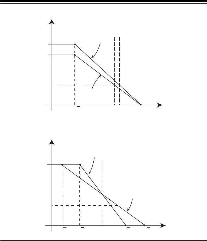
Figure 4 illustrates the fact that a ﬂatter demand curve for reserves is

associated with less volatility in the market interest rate, given a particular level

of uncertainty associated with autonomous factors. Suppose this uncertainty

implies that, after a given open market operation, the total supply of reserves

will be equal to either S or S



in the ﬁgure. With the steeper (thick) demand

curve, this uncertainty about the supply of reserves leads to a relatively wide

range of uncertainty about the market rate. With the ﬂatter (thin) demand

curve, in contrast, the variation in the market rate is smaller. For this reason,

the slope of the demand curve, and those policies that affect the slope, are

important determinants of the observed degree of volatility of the market

interest rate around the target.

As discussed in the previous section, a variety of factors affect the slope

of the aggregate demand for reserves. Figure 4 can be viewed, for example, as

comparing a situation where all banks face relatively little late-day uncertainty

with one where all banks face more uncertainty; the latter case corresponds

unaffected. The analysis also takes the size and timing of payments as given. Several papers have

studied the interesting question of how banks respond to incentives in choosing the timing of their

outgoing payments and, hence, their daylight credit usage. See, for example, McAndrews and

Rajan (2000) and Bech and Garratt (2003).

H. M. Ennis and T. Keister: Monetary Policy Implementation 251

Figure 4 Interest Rate Volatility

Low Volatility

High

Volatility

to the thin line in the ﬁgure. However, it should be clear that the reasoning

presented above does not depend on this particular interpretation. The exact

same results about interest rate volatility would obtain if the demand curves had

different slopes because banks face different penalty rates in the two scenarios

or because of some other factor(s). What the ﬁgure shows is that there is a

direct relationship between the slope of the demand curve and the amount of

interest rate volatility caused by forecast errors or other unanticipated changes

in the supply of reserves.

Central banks generally aim to limit the volatility of the interest rate around

their target level to the extent possible. For this reason, a variety of policy

arrangements have been designed in an attempt to decrease the slope of the

demand curve, at least in the region that is considered “relevant.” In the

remainder of the article, we show how some of these tools can be analyzed

in the context of our simple framework. In Section 4 we discuss reserve

maintenance periods, while in Section 5 we discuss approaches that become

feasible when the central bank pays interest on reserves.

4. RESERVE MAINTENANCE PERIODS

Perhaps the most signiﬁcant arrangement designed to ﬂatten the demand curve

for reserves is the introduction of reserve maintenance periods. In a system

252 Federal Reserve Bank of Richmond Economic Quarterly

with a reserve maintenance period, banks are not required to hold a particular

quantity of reserves each day. Rather, each bank is required to hold a certain

average level of reserves over the maintenance period. In the United States,

the length of the maintenance period is currently two weeks.

The presence of a reserve maintenance period gives banks some ﬂexibility

in determining when they hold reserves to meet their requirement. In general,

banks will try to hold more reserves on days in which they expect the market

interest rate to be lower and fewer reserves on days when they expect the rate

to be higher. This ﬂexibility implies that a bank’s reserve holdings will tend to

be more responsive to changes in the interest rate on any given day. In other

words, having a reserve maintenance period tends to make the demand curve

ﬂatter, at least on days prior to the last day of the maintenance period. We

illustrate this effect by studying a two-day maintenance period in the context

of the simple framework. We then brieﬂy explain how the same logic applies

to longer periods.

A Two-Day Maintenance Period

Let K denote the average daily requirement so that the total requirement for

the two-day maintenance period is 2K. The derivation of the demand curve

for reserves on the second (and ﬁnal) day of the maintenance period follows

exactly the same logic as in our benchmark case. The only difference with

Figure 1 is that the reserve requirement will be given by the amount of reserves

that the bank has left to hold in order to satisfy the requirement for the period.

In other words, the reserve requirement on the second day is equal to 2K

minus the quantity of reserves the bank held at the end of the ﬁrst day.

On the ﬁrst day of the maintenance period, a bank’s demand for reserves

depends crucially on its belief about what the market interest rate will be on the

second day. Suppose the bank expects the market interest rate on the second

day to equal the target rate, r

. Figure 5 depicts the demand for reserves on the

ﬁrst day under this assumption.

As in the basic case presented in Figure 1,

there would be no demand for reserves if the market interest rate were greater

than r

. Suppose instead that the market interest rate on the ﬁrst day is close

to, but smaller than, the penalty rate, r

. Then the bank will want to satisfy as

much of its reserve requirement as possible on the second day, when it expects

the rate to be substantially lower. However, if the bank’s reserve balance after

the late-day payment shock is negative, it will be forced to borrow funds at the

penalty rate to avoid incurring an overnight overdraft. As long as the market

rate is below the penalty rate, the bank will choose a reserve position of at least

−

P . Note that this reserve position represents the amount of reserves held by

For simplicity, Figure 5 is drawn with no discounting on the part of the bank. The effect

of discounting is very small and inessential for understanding the basic logic described here.

H. M. Ennis and T. Keister: Monetary Policy Implementation 253

Figure 5 A Two-Day Maintenance Period

2K-P 2K+P

the bank before the late-day payment shock is realized. Even if this position is

negative, as would be the case when the market rate is close to r

in Figure 5,

it is still possible that the bank will receive a late-day inﬂow of reserves such

that it does not need to borrow funds at the penalty rate to avoid an overnight

overdraft. However, if the bank were to choose a position smaller than −

P ,

it would be certain to need to borrow at the penalty rate, which cannot be an

optimal choice as long as the market rate is lower.

For interest rates below r

, but still larger than the target rate, the bank will

choose to hold some “precautionary” reserves to decrease the probability that

it will need to borrow at the penalty rate. This precautionary motive generates

the ﬁrst downward-sloping part of the demand curve in the ﬁgure. As long

as the day-one interest rate is above the target rate, however, the bank will

not hold more than

P in reserves on the ﬁrst day. By holding P , the bank is

assured that it will have a positive reserve balance after the late-day payment

shock. If the bank were holding more than

P on the ﬁrst day, it could lend

those reserves out at the (relatively high) market rate and meet its requirement

by borrowing reserves on the second day in the event that the interest rate is

expected to be at the (lower) target rate, yielding a positive proﬁt. Hence, the

ﬁrst downward-sloping part of the demand curve must end at

P .

Now suppose the ﬁrst-day interest rate is exactly equal to the target rate,

. In this case, the bank expects the rate to be the same on both days and is,

254 Federal Reserve Bank of Richmond Economic Quarterly

therefore, indifferent between holding reserves on either day for the purpose

of meeting reserve requirements. In choosing its ﬁrst-day reserve position, the

bank will consider the following issues. It will choose to hold at least enough

reserves to ensure that it will not need to borrow at the penalty rate at the end

of the ﬁrst day. In other words, reserve holdings will be at least as large as the

largest possible payment

P .

The bank is willing to hold more reserves than

P for the purpose of

satisfying some of its requirement. However, it wants to avoid the possi-

bility of over-satisfying the requirement on the ﬁrst day (that is, becoming

“locked-in”), since it must hold a non-negative quantity of reserves on the

second day to avoid an overnight overdraft. This implies that the bank will

not be willing to hold more than the total requirement, 2K, minus the largest

possible payment inﬂow,

P , on the ﬁrst day. The demand curve is ﬂat between

these two points (that is,

P and 2K − P ), indicating that the bank is indifferent

between the various levels of reserves in this interval.

Finally, suppose the market interest rate on the ﬁrst day is smaller than the

target rate. Then the bank wants to satisfy most of the requirement on the ﬁrst

day, since it expects the market rate to be higher on the second day. In this case,

the bank will hold at least 2K −

P reserves on the ﬁrst day. If it held any less

than this amount, it would be certain to have some requirement remaining on

the second day, which would not be an optimal choice given that the rate will

be higher on the second day. As the interest rate moves farther below the target

rate, the bank will hold more reserves for the usual precautionary reasons. In

this case, the bank is balancing the possibility of being locked-in after the

ﬁrst day against the possibility of needing to meet some of its requirement on

the more-expensive second day. The larger the difference between the rates

on the two days, the larger the quantity the bank will choose to hold on the

ﬁrst day. This trade-off generates the second downward-sloping part of the

demand curve.

The intermediate ﬂat portion of the demand curve in Figure 5 can help

to reduce the volatility of the interest rate on days prior to the settlement

day. As long as movements in autonomous factors are small enough such that

the supply of reserves stays in this portion of the demand curve, interest rate

ﬂuctuations will be minimal. For a central bank that is interested in minimizing

volatility around its target rate, this represents a substantial improvement over

the situation depicted in Figure 1.

It should be noted that Figure 5 is drawn under the assumption that the reserve requirement

is relatively large. Speciﬁcally, K>

P is assumed to hold, so that the total reserve requirement for

the period, 2K, is larger than the width of the support of the late-day payment shock, 2

P . If this

inequality were reserved, the ﬂat portion of the demand curve would not exist. In general, reserve

maintenance periods are most useful as a policy tool when the underlying reserve requirements

are sufﬁciently large relative to the end-of-day balance uncertainty.

H. M. Ennis and T. Keister: Monetary Policy Implementation 255

There are, however, some issues that make implementing the target rate

through reserve maintenance periods more difﬁcult than a simple interpreta-

tion of Figure 5 might suggest. First, the position of the ﬂat portion of the

demand curve at the exact level of the target rate depends on the central bank’s

ability to hit the target rate (on average) on settlement day. If banks expected

the settlement-day interest rate to be lower than the current target, for example,

the ﬂat portion of the ﬁrst-day demand curve would also lie below the target.

This issue is particularly problematic when market participants expect the cen-

tral bank’s target rate to change during the course of a reserve maintenance

period. A second difﬁculty is that the ﬂat portion of the demand curve disap-

pears on the settlement day and the curve reverts to that in Figure 1.

This

feature of the model indicates why market interest rates are likely to be more

volatile on settlement days.

Multiple-Day Maintenance Periods

Maintenance periods with three or more days can be easily analyzed in a

similar way. Consider, for example, the case of a three-day maintenance

period with an average daily requirement equal to K. As before, suppose that

the central bank is expected to hit the target rate on the subsequent days of the

maintenance period and consider the demand for reserves on the ﬁrst day. This

demand will be ﬂat between the points

P and 3K − P . That is, the demand

curve will be similar to that plotted in Figure 5, but the ﬂat portion will be

wider.

To determine the shape of the demand curve for reserves on the second

day we need to know how many reserves the bank held on the ﬁrst day of

the maintenance period. Suppose the bank held R

reserves with R

< 3K.

Then on the second day of the maintenance period, the demand curve for

reserves would be ﬂat between the points

P and 3K − R

− P . Hence, we see

that as the bank approaches the ﬁnal day of the maintenance period, the ﬂat

portion of its demand curve is likely to become smaller, potentially opening the

door to increases in interest rate volatility. For the interested reader, Bartolini,

Bertola, and Prati (2002) provide a more thorough analysis of the implications

of multiple-day maintenance periods on the behavior of the overnight market

interest rate using a model similar to, but more general than, ours.

In practice, central banks often use carryover provisions in an attempt to generate a small

ﬂat region in the demand curve on a settlement day. Another alternative would be to stagger the

reserve maintenance periods for different groups of banks. This idea goes back to as early as the

1960s (see, for example, the discussion between Sternlight 1964 and Cox and Leach 1964 in the

Journal of Finance). One common argument against staggering the periods is that it could make

the task of predicting reserve demand more difﬁcult. Whether the beneﬁts of reducing settlement

day variability outweigh the potential costs of staggering is difﬁcult to determine.

256 Federal Reserve Bank of Richmond Economic Quarterly

5. PAYING INTEREST ON RESERVES

We now introduce the possibility that the central bank pays interest on the

reserve balances held overnight by banks in their accounts at the central bank.

As discussed in Section 1, most central banks currently pay interest on reserves

in some form, and Congress has authorized the Federal Reserve to begin doing

so in October 2011. The ability to pay interest on reserves gives a central bank

an additional policy tool that can be used to help minimize the volatility of

the market interest rate and steer this rate to the target level. This tool can be

especially useful during periods of ﬁnancial distress. For example, during the

recent ﬁnancial turmoil, the fed funds rate has experienced increased volatility

during the day and has, in many cases, collapsed to values near zero late in

the day. As we will see below, the ability to pay interest on reserves allows

the central bank to effectively put a ﬂoor on the values of the interest rate that

can be observed in the market. Such a ﬂoor reduces volatility and potentially

increases the ability of the central bank to achieve its target rate.

In this section, we describe two approaches to monetary policy imple-

mentation that rely on paying interest on reserves: an interest rate corridor

and a system with clearing bands. We explain the basic components of each

approach and how each tends to ﬂatten the demand curve for reserves.

Interest Rate Corridors

One simple policy a central bank could follow would be to pay a ﬁxed interest

rate, r

, on all reserve balances that a bank holds in its account at the central

bank.

This policy places a ﬂoor on the market interest rate: No bank would

be willing to lend reserves at an interest rate lower than r

, since they could

instead earn r

by simply holding the reserves on deposit at the central bank.

Together, the penalty rate, r

, and the deposit rate, r

, form a “corridor” in

which the market interest rate will remain.

Figure 6 depicts the demand for reserves under a corridor system. As in

the earlier ﬁgures, there is no demand for reserves if the market interest rate is

higher than the penalty rate, r

. For values of the market interest rate below

, a bank will choose to hold at least K − P reserves for exactly the same

In practice, reserve balances held to meet requirements are often compensated at a different

rate than those that are held in excess of a bank’s requirement. For the daily process of targeting

the overnight market interest rate, the rate paid on excess reserves is what matters; this is the rate

we denote r

in our analysis.

A central bank may prefer to use a lending facility that is distinct from its discount window

to form the upper bound of the corridor. Banks may be reluctant to borrow from the discount

window, which serves as a lender of last resort, because they fear that others would interpret this

borrowing as a sign of poor ﬁnancial health. The terms associated with the lending facility could

be designed to minimize this type of stigma effect and, thus, create a more reliable upper bound

on the market interest rate.

H. M. Ennis and T. Keister: Monetary Policy Implementation 257

Figure 6 A Conventional Corridor

K-P

K+P R

Demand for

Reserves

reason as in Figure 1: if it held a lower level of reserves, it would be certain to

need to borrow at the penalty rate, r

. Also as before, the demand for reserves

is downward-sloping in this region. The big change from Figure 1 is that the

demand curve now becomes ﬂat at the deposit rate. If the market rate were

lower than the deposit rate, a bank’s demand for reserves would be essentially

inﬁnite, as it would try to borrow at the market rate and earn a proﬁt by simply

holding the reserves overnight.

The ﬁgure shows that, regardless of the level of reserve supply, S, the

market interest rate will always stay in the corridor formed by the rates r

and r

. The width of the corridor, r

− r

, is then a policy choice. Choosing

a relatively narrow corridor will clearly limit the range and volatility of the

market interest rate. Note that narrowing the corridor also implies that the

downward-sloping part of the demand curve becomes ﬂatter (to see this, notice

that the boundary points K −

P and K + P do not depend on r

or r

Hence, the size of the interest rate movement associated with a given shock

to an autonomous factor is smaller, even when the shock is small enough to

keep the rate within the corridor.

An interesting case to consider is one in which the lending and deposit

rates are set the same distance on either side of the target rate (x basis points

above and below the target, respectively). This system is called a symmetric

258 Federal Reserve Bank of Richmond Economic Quarterly

corridor. A change in policy stance that involves increasing the target rate,

then, effectively amounts to changing the levels of the lending and deposit

rates, which shifts the demand curve along with them. The supply of reserves

needed to maintain a higher target rate, for example, may not be lower. In

fact— perhaps surprisingly—in the simple model studied here, the target level

of the supply of reserves would not change at all when the policy rate changes.

If the demand curve in Figure 6 is too steep to allow the central bank to

effectively achieve its goal of keeping the market rate close to the target, a

corridor system could be combined with a reserve maintenance period of the

type described in Section 4. The presence of a reserve maintenance period

would generate a ﬂat region in the demand curve as in Figure 5. The features of

the corridor would make the two downward-sloping parts of the demand curve

in Figure 5 less steep, which would limit the interest rate volatility associated

with events where reserve supply exits the ﬂat region of the demand curve, as

well as on the last day of the maintenance period when the ﬂat region is not

present.

Another way to limit interest rate volatility is for the central bank to set the

deposit rate equal to the target rate and then provide enough reserves to make

the supply, S

, intersect the demand curve well into the ﬂat portion of the

demand curve at rate r

. This “ﬂoor system” has been recently advocated as a

way to simplify monetary policy implementation (see, for example, Woodford

2000, Goodfriend 2002, and Lacker 2006). Note that such a system does

not rely on a reserve maintenance period to generate the ﬂat region of the

demand curve, nor does it rely on reserve requirements to induce banks to

hold reserves. To the extent that reserve requirements, and the associated

reporting procedures, place signiﬁcant administrative burdens on both banks

and the central bank, setting the ﬂoor of the corridor at the target rate and

simplifying, or even eliminating, reserve requirements could potentially be an

attractive system for monetary policy implementation.

It should be noted, however, that the market interest rate will always

remain some distance above the ﬂoor in such a system, since lenders in the

market must be compensated for transactions costs and for assuming some

counterparty credit risk. In other words, in a ﬂoor system the central bank is

able to fully control the risk-free interest rate, but not necessarily the market

rate. In normal times, the gap between the market rate and the rate paid on

reserves would likely be stable and small. In periods of ﬁnancial distress,

however, elevated credit risk premia may drive the average market interest

rate signiﬁcantly above the interest rate paid on reserves. Our simple model

abstracts from these important considerations.

The central bank could also set an upper limit for the quantity of reserves on which it

would pay the target rate of interest to a bank; reserves above this limit would earn a lower

rate (possibly zero). Whitesell (2006) proposed that banks be allowed to choose their own upper

H. M. Ennis and T. Keister: Monetary Policy Implementation 259

Clearing Bands

Another approach to generating a ﬂat region in the demand curve for re-

serves is the use of daily clearing bands. This approach does not rely on a

reserve maintenance period. Instead, the central bank pays interest on a bank’s

reserve holdings at the target rate, r

, as long as those holdings fall within a

pre-speciﬁed band. Let K

and K denote the lower and upper bounds of this

band, respectively. If the bank’s reserve balance falls below K

, it must borrow

at the penalty rate, r

, to bring its balance up to at least K. If, on the other

hand, the bank’s reserve balance is higher than

K, it will earn the target rate,

, on all balances up to K but will earn a lower rate, r

, beyond that bound.

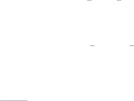
The demand curve for reserves under such a system is depicted in Figure

7. The ﬁgure is drawn under the assumption that the clearing band is fairly

wide relative to the support of the late-day payment shock. In particular, we

assume that K

+ P<K − P . Let us call the interval



K + P,K − P



the

“intermediate region” for reserves. By choosing any level of reserves in this

intermediate region, a bank can ensure that its end-of-day reserve balance will

fall within the clearing band. The bank would then be sure that it will earn the

target rate of interest on all of the reserves it ends up holding overnight.

When the market interest rate is equal to the target rate, r

, a bank is

indifferent between choosing any level of reserves in the intermediate region.

For example, if the bank borrows in the market to slightly increase its reserve

holdings, the cost it would pay in the market for those reserves would be exactly

offset by the extra interest it would earn from the central bank. Similarly,

lending out reserves to slightly decrease the bank’s holdings would also leave

proﬁt unchanged. This reasoning shows that the demand curve for reserves

will be ﬂat in the intermediate region between K

+ P and K − P . As long as

the central bank is able to keep the supply of reserves within this region, the

market interest rate will equal the target rate, r

, regardless of the exact level

of reserve supply.

Outside the intermediate region, the logic behind the shape of the demand

curve is very similar to that explained in our benchmark case. When the market

interest rate is higher than r

, a bank can earn more by lending reserves in

the market than by holding them on deposit at the central bank. It would,

therefore, prefer not to hold more than the minimum level of reserves needed

to avoid being penalized, K

. Of course, the bank would be willing to hold

some precautionary reserves to guard against the possibility that the late-

day payment shock will drive their reserve balance below K

. The quantity of

precautionary reserves it would choose to hold is, as before, an inverse function

of the market interest rate; this reasoning generates the ﬁrst downward-sloping

part of the demand curve in Figure 7.

limits by paying a facility fee per unit of capacity. Such an approach leads to a demand curve

for reserves that is ﬂat at the target rate over a wide region.

260 Federal Reserve Bank of Richmond Economic Quarterly

Figure 7 A Clearing Band

K-P

K+P

When the market rate is below r

, on the other hand, the bank would like

to take full advantage of its ability to earn the target interest rate by holding

reserves at the central bank. It would, however, take into consideration the

possibility that a late-day inﬂow of funds will leave it with a ﬁnal balance

higher than

K, in which case it would earn the lower interest rate, r

, on the

excess funds. The resulting decision process generates a downward-sloping

region of the demand curve between the rates r

and r

. As in Figure 6, the

demand curve never falls below the interest rate paid on excess reserves (now

labeled r

); thus, this rate creates a ﬂoor for the market interest rate.

The demand curve in Figure 7 has the same basic shape as the one gen-

erated by a reserve maintenance period, which was depicted in Figure 5. It is

important to keep in mind, however, that the forces generating the ﬂat portion

of the demand curve in the intermediate region are fundamentally different in

the two cases. The reserve maintenance period approach relies on intertem-

poral arbitrage: banks will want to hold more reserves on days when the

market interest rate is low and fewer reserves when the market rate is high.

This activity will tend to equate the current market interest rate to the expected

future rate (as long as the supply of reserves is in the intermediate region).

The clearing band system relies instead on intraday arbitrage to generate the

ﬂat portion of the demand curve: banks will want to hold more reserves when

H. M. Ennis and T. Keister: Monetary Policy Implementation 261

the market interest rate is low, for example, simply to earn the higher interest

rate paid by the central bank.

The intertemporal aspect of reserve maintenance periods has two clear

drawbacks. First, if—for whatever reason—the expected future rate differs

from the target rate, r

, it becomes difﬁcult for the central bank to achieve the

target rate in the current period. Second, large shocks to the supply of reserves

on one day can have spillover effects on subsequent days in the maintenance

period. If, for example, the supply of reserves is unusually high one day, banks

will satisfy an unusually large portion of their reserve requirements and, as a

result, the ﬂat portion of the demand curve will be smaller on all subsequent

days, increasing the potential for rate volatility on those days.

The clearing band approach, in contrast, generates a ﬂat portion in the

demand curve that always lies at the current target interest rate, even if market

participants expect the target rate to change in the near future. Moreover,

the width of the ﬂat portion is “reset” every day; it does not depend on past

events. These features are important potential advantages of the clearing band

approach. We should again point out, however, that our simple model has

abstracted from transaction costs and credit risk. As with the ﬂoor system dis-

cussed above, these considerations could result in the average market interest

rate being higher than the rate r

, as the latter represents a risk-free rate.

6. CONCLUSION

A recent change in legislation that allows the Federal Reserve to pay interest on

reserves has renewed interest in the debate over the most effective way to im-

plement monetary policy. In this article, we have provided a basic framework

that can be useful for analyzing the main properties of the various alterna-

tives. While we have conducted all our analysis graphically, our simplifying

assumptions permit a fairly precise description of the alternatives and their

effectiveness at implementing a target interest rate.

Many extensions of our basic framework are possible and we have ana-

lyzed several of them in this article. However, some important issues remain

unexplored. For example, we only brieﬂy mentioned the difﬁculties that ﬂuc-

tuations in aggregate credit risk can introduce in the implementation process.

Also, as the debate continues, new questions will arise. We believe that the

framework introduced in this article can be a useful ﬁrst step in the search for

much-needed answers.

262 Federal Reserve Bank of Richmond Economic Quarterly

REFERENCES

Ashcraft, Adam, James McAndrews, and David Skeie. 2007. “Precautionary

Reserves and the Interbank Market.” Mimeo, Federal Reserve Bank of

New York (July).

Bartolini, Leonardo, Giuseppe Bertola, and Alessandro Prati. 2002.

“Day-To-Day Monetary Policy and the Volatility of the Federal Funds

Interest Rate.” Journal of Money, Credit, and Banking 34 (February):

137–59.

Bech, M. L., and Rod Garratt. 2003. “The Intraday Liquidity Management

Game.” Journal of Economic Theory 109 (April): 198–219.

Clouse, James A., and James P. Dow, Jr. 2002. “A Computational Model of

Banks’ Optimal Reserve Management Policy.” Journal of Economic

Dynamics and Control 26 (September): 1787–814.

Cox, Albert H., Jr., and Ralph F. Leach. 1964. “Open Market Operations and

Reserve Settlement Periods: A Proposed Experiment.” Journal of

Finance 19 (September): 534–9.

Coy, Peter. 2007. “A ‘Stealth Easing’ by the Fed?” BusinessWeek.

http://www.businessweek.com/investor/content/aug2007/

pi20070817

445336.htm [17 August].

Dotsey, Michael. 1991. “Monetary Policy and Operating Procedures in New

Zealand.” Federal Reserve Bank of Richmond Economic Review

(September/October): 13–9.

Ennis, Huberto M., and John A. Weinberg. 2007. “Interest on Reserves and

Daylight Credit.” Federal Reserve Bank of Richmond Economic

Quarterly 93 (Spring): 111–42.

Goodfriend, Marvin. 2002. “Interest on Reserves and Monetary Policy.”

Federal Reserve Bank of New York Economic Policy Review 8 (May):

77–84.

Guthrie, Graeme, and Julian Wright. 2000. “Open Mouth Operations.”

Journal of Monetary Economics 46 (October): 489–516.

Hilton, Spence, and Warren B. Hrung. 2007. “Reserve Levels and Intraday

Federal Funds Rate Behavior.” Federal Reserve Bank of New York Staff

Report 284 (May).

Keister, Todd, Antoine Martin, and James McAndrews. 2008. “Divorcing

Money from Monetary Policy.” Federal Reserve Bank of New York

Economic Policy Review 14 (September): 41–56.

H. M. Ennis and T. Keister: Monetary Policy Implementation 263

Lacker, Jeffrey M. 2006. “Central Bank Credit in the Theory of Money and

Payments.” Speech. http://www.richmondfed.org/news

and speeches/

presidents

speeches/index.cfm/2006/id=88/pdf=true.

McAndrews, James, and Samira Rajan. 2000. “The Timing and Funding of

Fedwire Funds Transfers.” Federal Reserve Bank of New York

Economic Policy Review 6 (July): 17–32.

Poole, William. 1968. “Commercial Bank Reserve Management in a

Stochastic Model: Implications for Monetary Policy.” Journal of

Finance 23 (December): 769–91.

Sternlight, Peter D. 1964. “Reserve Settlement Periods of Member Banks:

Comment.” Journal of Finance 19 (March): 94–8.

Whitesell, William. 2006. “Interest Rate Corridors and Reserves.” Journal of

Monetary Economics 53 (September): 1177–95.

Woodford, Michael. 2000. “Monetary Policy in a World Without Money.”

International Finance 3 (July): 229–60.