
Recommendation ITU-R BT.500-13
(01/2012)
Methodology for the subjective
assessment of the quality
of television pictures
BT Series
Broadcasting service
(television)

ii Rec. ITU-R BT.500-13
Foreword
The role of the Radiocommunication Sector is to ensure the rational, equitable, efficient and economical use of the
radio-frequency spectrum by all radiocommunication services, including satellite services, and carry out studies without
limit of frequency range on the basis of which Recommendations are adopted.
The regulatory and policy functions of the Radiocommunication Sector are performed by World and Regional
Radiocommunication Conferences and Radiocommunication Assemblies supported by Study Groups.
Policy on Intellectual Property Right (IPR)
ITU-R policy on IPR is described in the Common Patent Policy for ITU-T/ITU-R/ISO/IEC referenced in Annex 1 of
Resolution ITU-R 1. Forms to be used for the submission of patent statements and licensing declarations by patent
holders are available from http://www.itu.int/ITU-R/go/patents/en where the Guidelines for Implementation of the
Common Patent Policy for ITU-T/ITU-R/ISO/IEC and the ITU-R patent information database can also be found.
Series of ITU-R Recommendations
(Also available online at http://www.itu.int/publ/R-REC/en)
Series
Title
BO
Satellite delivery
BR
Recording for production, archival and play-out; film for television
BS
Broadcasting service (sound)
BT Broadcasting service (television)
F
Fixed service
M
Mobile, radiodetermination, amateur and related satellite services
P
Radiowave propagation
RA
Radio astronomy
RS
Remote sensing systems
S
Fixed-satellite service
SA
Space applications and meteorology
SF
Frequency sharing and coordination between fixed-satellite and fixed service systems
SM
Spectrum management
SNG
Satellite news gathering
TF
Time signals and frequency standards emissions
V
Vocabulary and related subjects
Note: This ITU-R Recommendation was approved in English under the procedure detailed in Resolution ITU-R 1.
Electronic Publication
Geneva, 2012
ITU 2012
All rights reserved. No part of this publication may be reproduced, by any means whatsoever, without written permission of ITU.
Rec. ITU-R BT.500-13 1
RECOMMENDATION ITU-R BT.500-13
Methodology for the subjective assessment of the quality
of television pictures
(Question ITU-R 81/6)
(1974-1978-1982-1986-1990-1992-1994-1995-1998-1998-2000-2002-2009-2012)
Scope
This Recommendation provides methodologies for the assessment of picture quality including general
methods of test, the grading scales and the viewing conditions. It recommends the double-stimulus
impairment scale (DSIS) method and the double-stimulus continuous quality-scale (DSCQS) method as well
as alternative assessment methods such as single-stimulus (SS) methods, stimulus-comparison methods,
single stimulus continuous quality evaluation (SSCQE) and simultaneous double stimulus for continuous
evaluation (SDSCE) method.
The ITU Radiocommunication Assembly,
considering
a) that a large amount of information has been collected about the methods used in various
laboratories for the assessment of picture quality;
b) that examination of these methods shows that there exists a considerable measure of
agreement between the different laboratories about a number of aspects of the tests;
c) that the adoption of standardized methods is of importance in the exchange of information
between various laboratories;
d) that routine or operational assessments of picture quality and/or impairments using a
five-grade quality and impairment scale made during routine or special operations by certain
supervisory engineers, can also make some use of certain aspects of the methods recommended for
laboratory assessments;
e) that the introduction of new kinds of television signal processing such as digital coding and
bit-rate reduction, new kinds of television signals using time-multiplexed components and, possibly,
new services such as enhanced television and HDTV may require changes in the methods of
making subjective assessments;
f) that the introduction of such processing, signals and services, will increase the likelihood
that the performance of each section of the signal chain will be conditioned by processes carried out
in previous parts of the chain,
recommends
1 that the general methods of test, the grading scales and the viewing conditions for the
assessment of picture quality, described in the following Annexes should be used for laboratory
experiments and whenever possible for operational assessments;
2 that, in the near future and notwithstanding the existence of alternative methods and the
development of new methods, those described in § 4 and 5 of Annex 1 to this Recommendation
should be used when possible; and
2 Rec. ITU-R BT.500-13
3 that, in view of the importance of establishing the basis of subjective assessments, the
fullest descriptions possible of test configurations, test materials, observers, and methods should be
provided in all test reports;
4 that, in order to facilitate the exchange of information between different laboratories, the
collected data should be processed in accordance with the statistical techniques detailed in Annex 2
to this Recommendation.
NOTE 1 – Information on subjective assessment methods for establishing the performance of
television systems is given in Annex 1.
NOTE 2 – Description of statistical techniques for the processing of the data collected during the
subjective tests is given in Annex 2.
Annex 1
Description of assessment methods
1 Introduction
Subjective assessment methods are used to establish the performance of television systems using
measurements that more directly anticipate the reactions of those who might view the systems
tested. In this regard, it is understood that it may not be possible to fully characterize system
performance by objective means; consequently, it is necessary to supplement objective
measurements with subjective measurements.
In general, there are two classes of subjective assessments. First, there are assessments that establish
the performance of systems under optimum conditions. These typically are called quality
assessments. Second, there are assessments that establish the ability of systems to retain quality
under non-optimum conditions that relate to transmission or emission. These typically are called
impairment assessments.
To conduct appropriate subjective assessments, it is first necessary to select from the different
options available those that best suit the objectives and circumstances of the assessment problem at
hand. To help in this task, after the general features reported in § 2, some information is given in § 3
on the assessment problems addressed by each method. Then, the two main recommended methods
are detailed in § 4 and 5. Finally, general information on alternative methods under study is reported
in § 6.
The purpose of this Annex is limited to the detailed description of the assessment methods. The
choice of the most appropriate method is nevertheless dependent on the service objectives the
system under test aims at. The complete evaluation procedures of specific applications are therefore
reported in other ITU-R Recommendations.
2 Common features
General viewing conditions for subjective assessments are given. Specific viewing conditions, for
subjective assessments of specific systems, are given in the related Recommendations.
2.1 General viewing conditions
Different environments with different viewing conditions are described.
Rec. ITU-R BT.500-13 3
The laboratory viewing environment is intended to provide critical conditions to check systems.
General viewing conditions for subjective assessments in the laboratory environment are given in
§ 2.1.1.
The home viewing environment is intended to provide a means to evaluate quality at the consumer
side of the TV chain. General viewing conditions in § 2.1.2 reproduce a near to home environment.
These parameters have been selected to define an environment slightly more critical than the typical
home viewing situations.
Some aspects relating to the monitors resolution and contrast are discussed.
2.1.1 Laboratory environment
2.1.1.1 General viewing conditions for subjective assessments in laboratory environment
The assessors’ viewing conditions should be arranged as follows:
a) Ratio of luminance of inactive screen to peak luminance: ≤ 0.02
b) Ratio of the luminance of the screen, when displaying
only black level in a completely dark room, to that
corresponding to peak white: ≈ 0.01
c) Display brightness and contrast: set up via PLUGE
(see Recommendations
ITU-R BT.814 and
ITU-R BT.815)
d) Maximum observation angle relative to the normal (this number
applies to CRT displays, whereas the appropriate numbers for
other displays are under study): 30°
e) Ratio of luminance of background behind picture monitor to
peak luminance of picture: ≈ 0.15
f) Chromaticity of background: D
65
g) Other room illumination: low
2.1.2 Home environment
2.1.2.1 General viewing conditions for subjective assessments in home environment
a) Ratio of luminance of inactive screen to peak luminance: ≤ 0.02 (see § 2.1.4)
b) Display brightness and contrast: set up via PLUGE
(see Recommendations
ITU-R BT.818 and
ITU-R BT.815)
c) Maximum observation angle relative to the normal
(this number applies to CRT displays, whereas the
appropriate numbers for other displays are under study): 30°
d) Screen size for a 4/3 format ratio: This screen size should
satisfy rules of preferred
viewing distance (PVD)
e) Screen size for a 16/9 format ratio: This screen size should
satisfy PVD rules
4 Rec. ITU-R BT.500-13
f) Monitor processing: Without digital
processing
g) Monitor resolution: See § 2.1.3
h) Peak luminance: 200 cd/m
2
i) Environmental illuminance on the screen (Incident
light from the environment falling on the screen,
should be measured perpendicularly to the screen): 200 lux
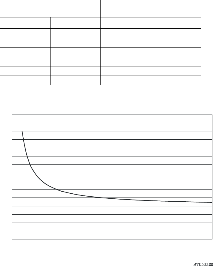
The viewing distance and the screen sizes are to be selected in order to satisfy the PVD. The PVD
(in function of the screen sizes) is shown in the following table and graph. Figures could be valid
both for SDTV and HDTV as very little difference was found.
15
14
13
12
11
10
9
8
7
6
5
4
3
2
1
0
PVD for moving image
s
P
V
D
()
Ratio of viewing distance (m) to picture height (m)
H
0 0.5 1 1.5 2
Screen height (m)
This table and graph are intended to give information on the PVD and related screen sizes to be
adopted in the Recommendations for specific applications.
Screen diagonal
(in)
Screen height
(H )
PVD
4/3 ratio 16/9 ratio (m) (H )
12 15 0.18 9
15 18 0.23 8
20 24 0.30 7
29 36 0.45 6
60 73 0.91 5
> 100 > 120 > 1.53 3-4

Rec. ITU-R BT.500-13 5
2.1.3 Monitor resolution
The resolution of professional monitors, equipped with professional CRTs, usually complies with
the required standards for subjective assessments in their luminance operating range.
Not all monitors can reach a 200 cd/m
2
peak luminance.
To check and report the maximum and minimum resolutions (centre and corners of the screen) at
the used luminance value might be suggested.
If consumer TV sets with consumer CRTs are used for subjective assessments, the resolution could
be inadequate, depending on the luminance value.
In this case it is strongly recommended to check and report the maximum and minimum resolutions
(centre and corners of the screen) at the used luminance value.
At present the most practical system available to subjective assessments performers, in order to
check monitors or consumer TV sets resolution, is the use of a swept test pattern electronically
generated.
A visual analysis allows to check the resolution. The visual threshold is estimated to be –12/–20 dB.
The main drawback of this system is the aliasing created by the shadow mask that makes the visual
evaluation hard, but, on the other hand, the aliasing presence indicates that the video frequency
signal exceeds the limits given by the shadow mask, which under samples the video signal.
Further studies on CRTs definition testing could be recommended.
2.1.4 Monitor contrast
Contrast could be strongly influenced by the environment illuminance.
Professional monitors CRTs seldom use technologies to improve their contrast in a high
illuminance environment, so it is possible they do not comply with the requested contrast standard
if used in a high illuminance environment.
Consumer CRTs use technologies to get a better contrast in a high illuminance environment.
To calculate the contrast of a given CRT, the screen reflection coefficient, K, of such CRT is
needed. In the best case the screen reflection coefficient is approximately K = 6%.
With a diffused environment I illuminance of 200 lux and a K = 6%, a 3.82 cd/m
2
, luminance
reflection of inactive screen areas is calculated
with the following formula:
K
I
L
reflected
π
=
With the given values, the reflected luminance (cd/m
2
) is nearly 2% of the incident illuminance
(lux).
The CRT is considered not to have mirror like reflections on the front glass, whose exact influence
on contrast is difficult to quantify because it is very dependant on lighting conditions.
In § 2.1.1 and 2.1.2, the contrast ratio CR is expressed as:
maxmin
LLCR / =
6 Rec. ITU-R BT.500-13
where:
L
min
: luminance of inactive areas under ambient illumination (cd/m
2
) (with the given
values L
min
= L
inactive areas
+ L
reflected
= 3.82 cd/m
2
)
L
max
: luminance of white areas under ambient illumination (cd/m
2
) (with the given
values L
max
= L
white
+ L
reflected
= 200 + 3.82 cd/m
2
).
With such values a CR = 0.018 is computed, strictly close to the 0.02 value stated in § 2.1.1.1 and
2.1.2.1, a).
2.2 Source signals
The source signal provides the reference picture directly, and the input for the system under test. It
should be of optimum quality for the television standard used. The absence of defects in the
reference part of the presentation pair is crucial to obtain stable results.
Digitally stored pictures and sequences are the most reproducible source signals, and these are
therefore the preferred type. They can be exchanged between laboratories, to make system
comparisons more meaningful. Video or computer tapes are possible formats.
In the short term, 35 mm slide-scanners provide a preferred source for still pictures. The resolution
available is adequate for evaluation of conventional television. The colorimetry and other
characteristics of film may give a different subjective appearance to studio camera pictures. If this
affects the results, direct studio sources should be used, although this is often much less convenient.
As a general rule, slide-scanners should be adjusted picture by picture for best possible subjective
picture quality, since this would be the situation in practice.
Assessments of downstream processing capacity are often made with colour-matte. In studio
operations, colour-matte is very sensitive to studio lighting. Assessments should therefore
preferably use a special colour-matte slide pair, which will consistently give high-quality results.
Movement can be introduced into the foreground slide if needed.
It will be frequently required to take account of the manner in which the performance of the system
under test may be influenced by the effect of any processing that may have been carried out at an
earlier stage in the history of the signal. It is therefore desirable that whenever testing is carried out
on sections of the chain that may introduce processing distortions, albeit non-visible, the resulting
signal should be transparently recorded, and then made available for subsequent tests downstream,
when it is desired to check how impairments due to cascaded processing may accumulate along the
chain. Such recordings should be kept in the library of test material, for future use as necessary, and
include with them a detailed statement of the history of the recorded signal.
2.3 Selection of test materials
A number of approaches have been taken in establishing the kinds of test material required in
television assessments. In practice, however, particular kinds of test materials should be used to
address particular assessment problems. A survey of typical assessment problems and of test
materials used to address these problems is given in Table 1.

Rec. ITU-R BT.500-13 7
TABLE 1
Selection of test material*
Some parameters may give rise to a similar order of impairments for most pictures or sequences. In
such cases, results obtained with a very small number of pictures or sequences (e.g. two) may still
provide a meaningful evaluation.
However, new systems frequently have an impact which depends heavily on the scene or sequence
content. In such cases, there will be, for the totality of programme hours, a statistical distribution of
impairment probability and picture or sequence content. Without knowing the form of this
distribution, which is usually the case, the selection of test material and the interpretation of results
must be done very carefully.
In general, it is essential to include critical material, because it is possible to take this into account
when interpreting results, but it is not possible to extrapolate from non-critical material. In cases
where scene or sequence content affects results, the material should be chosen to be “critical but not
unduly so” for the system under test. The phrase “not unduly so” implies that the pictures could still
conceivably form part of normal programme hours. At least four items should, in such cases, be
used: for example, half of which are definitely critical, and half of which are moderately critical.
A number of organizations have developed test still pictures and sequences. It is hoped to organize
these in the framework of the ITU-R in the future. Specific picture material is proposed in the
Recommendations addressing the evaluation of the applications.
Further ideas on the selection of test materials are given in Appendices 1 and 2 to Annex 1.
2.4 Range of conditions and anchoring
Because most of the assessment methods are sensitive to variations in the range and distribution of
conditions seen, judgement sessions should include the full ranges of the factors varied. However,
this may be approximated with a more restricted range, by presenting also some conditions that
would fall at the extremes of the scales. These may be represented as examples and identified as
most extreme (direct anchoring) or distributed throughout the session and not identified as most
extreme (indirect anchoring).
Assessment problem Material used
Overall performance with average material General, “critical but not unduly so”
Capacity, critical applications (e.g. contribution,
post-processing, etc.)
Range, including very critical material for the application tested
Performance of “adaptive” systems Material very critical for “adaptive” scheme used
Identify weaknesses and possible improvements Critical, attribute-specific material
Identify factors on which systems are seen to vary Wide range of very rich material
Conversion among different standards Critical for differences (e.g. field rate)
* It is understood that all test materials could conceivably be part of television programme content. For further guidance on the
selection of test materials, see Appendices 1 and 2 to Annex 1.
8 Rec. ITU-R BT.500-13
2.5 Observers
Observers may be expert or non-expert depending on the objectives of the assessment. An expert
observer is an observer that has expertise in the image artefacts that may be introduced by the
system under test. A non-expert (“naive”) observer is an observer that has no expertise in the image
artefacts that may be introduced by the system under test. In any case, observers should not be, or
have been, directly involved, i.e., enough to acquire specific and detailed knowledge, in the
development of the system under study.
Prior to a session, the observers should be screened for (corrected-to-) normal visual acuity on the
Snellen or Landolt chart, and for normal colour vision using specially selected charts (Ishihara, for
instance). At least 15 observers should be used. The number of assessors needed depends upon the
sensitivity and reliability of the test procedure adopted and upon the anticipated size of the effect
sought. For studies with limited scope, e.g., of exploratory nature, fewer than 15 observers may be
used. In this case, the study should be identified as “informal”. The level of expertise in television
picture quality assessment of the observers should be reported.
A study of consistency between results at different testing laboratories has found that systematic
differences can occur between results obtained from different laboratories. Such differences will be
particularly important if it is proposed to aggregate results from several different laboratories in
order to improve the sensitivity and reliability of an experiment.
A possible explanation for the differences between different laboratories is that there may be
different skill levels amongst different groups of assessors. Further research needs to be undertaken
to assess the validity of this hypothesis and, if proven, to quantify the variations contributed by this
factor. However, in the interim, experimenters should include as much detail as possible on the
characteristics of their assessment panels to facilitate further investigation of this factor. Suggested
data to be provided could include: occupation category (e.g. broadcast organization employee,
university student, office worker, ...), gender, and age range.
2.6 Instructions for the assessment
Assessors should be carefully introduced to the method of assessment, the types of impairment or
quality factors likely to occur, the grading scale, the sequence and timing. Training sequences
demonstrating the range and the type of the impairments to be assessed should be used with
illustrating pictures other than those used in the test, but of comparable sensitivity. In the case of
quality assessments, quality may be defined as to consist of specific perceptual attributes.
2.7 The test session
A session should last up to half an hour. At the beginning of the first session, about five “dummy
presentations” should be introduced to stabilize the observers’ opinion. The data issued from these
presentations must not be taken into account in the results of the test. If several sessions are
necessary, about three dummy presentations are only necessary at the beginning of the following
session.
A random order should be used for the presentations (for example, derived from Graeco-Latin
squares); but the test condition order should be arranged so that any effects on the grading of
tiredness or adaptation are balanced out from session to session. Some of the presentations can be
repeated from session to session to check coherence.

Rec. ITU-R BT.500-13 9
FIGURE 1
Presentation structure of test session
Stabilizing
sequence(s)
(results for these items
are not processed)
Main part of test session
Training
sequence(s)
Break
(to allow time to answer
questions from observers)
2.8 Presentation of the results
Because they vary with range, it is inappropriate to interpret judgements from most of the
assessment methods in absolute terms (e.g. the quality of an image or image sequence).
For each test parameter, the mean and 95% confidence interval of the statistical distribution of the
assessment grades must be given. If the assessment was of the change in impairment with a
changing parameter value, curve-fitting techniques should be used. Logistic curve-fitting and
logarithmic axis will allow a straight line representation, which is the preferred form of
presentation. More information on data processing is given in Annex 2 to this Recommendation.
The results must be given together with the following information:
– details of the test configuration;
– details of the test materials;
– type of picture source and display monitors (see Note 1);
– number and type of assessors (see Note 2);
– reference systems used;
– the grand mean score for the experiment;
– original and adjusted mean scores and 95% confidence interval if one or more observers
have been eliminated according to the procedure given below.
NOTE 1 – Because there is some evidence that display size may influence the results of subjective
assessments, experimenters are requested to explicitly report the screen size, and make and model number of
displays used in any experiments.
NOTE 2 – There is evidence that variations in the skill level of viewing panels (even amongst non-expert
panels) can influence the results of subjective viewing assessments. To facilitate further study of this factor
experimenters are requested to report as much of the characteristics of their viewing panels as possible.
Relevant factors might include: the age and gender composition of the panel or the education or employment
category of the panel.
3 Selection of test methods
A wide variety of basic test methods have been used in television assessments. In practice, however,
particular methods should be used to address particular assessment problems. A survey of typical
assessment problems and of methods used to address these problems is given in Table 2.

10 Rec. ITU-R BT.500-13
TABLE 2
Selection of test methods
4 The double-stimulus impairment scale (DSIS) method (the EBU method)
4.1 General description
A typical assessment might call for an evaluation of either a new system, or the effect of a
transmission path impairment. The initial steps for the test organizer would include the selection of
sufficient test material to allow a meaningful evaluation to be made, and the establishment of which
test conditions should be used. If the effect of parameter variation is of interest, it is necessary to
choose a set of parameter values which cover the impairment grade range in a small number of
roughly equal steps. If a new system, for which the parameter values cannot be so varied, is being
evaluated, then either additional, but subjectively similar, impairments need to be added, or another
method such as that in § 5 should be used.
The double-stimulus (EBU) method is cyclic in that the assessor is first presented with an
unimpaired reference, then with the same picture impaired. Following this, he is asked to vote on
the second, keeping in mind the first. In sessions, which last up to half an hour, the assessor is
presented with a series of pictures or sequences in random order and with random impairments
covering all required combinations. The unimpaired picture is included in the pictures or sequences
to be assessed. At the end of the series of sessions, the mean score for each test condition and test
picture is calculated.
The method uses the impairment scale, for which it is usually found that the stability of the results
is greater for small impairments than for large impairments. Although the method sometimes has
been used with limited ranges of impairments, it is more properly used with a full range of
impairments.
Assessment problem Method used Description
Measure the quality of systems relative to a
reference
Double-stimulus continuous quality-scale
(DSCQS) method
(1)
Rec. ITU-R BT.500, § 5
Measure the robustness of systems (i.e. failure
characteristics)
Double-stimulus impairment scale (DSIS)
method
(1)
Rec. ITU-R BT.500, § 4
Quantify the quality of systems (when no
reference is available)
Ratio-scaling method
(2)
or categorical scaling
(under study)
Report ITU-R BT.1082
Compare the quality of alternative systems
(when no reference is available)
Method of direct comparison, ratio-scaling
method
(2)
or categorical scaling (under study)
Report ITU-R BT.1082
Identify factors on which systems are perceived
to differ and measure their perceptual influence
Method under study Report ITU-R BT.1082
Establish the point at which an impairment
becomes visible
Threshold estimation by forced-choice method
or method of adjustment (under study)
Report ITU-R BT.1082
Determine whether systems are perceived to
differ
Forced-choice method (under study) Report ITU-R BT.1082
Measure the quality of stereoscopic image
coding
Double stimulus continuous quality-scale
(DSCQS) method
(3)
Rec. ITU-R BT.500, § 5
Measure the fidelity between two impaired
video sequences
Simultaneous double stimulus for continuous
evaluation (SDSCE) method
Rec. ITU-R BT.500, § 6.4
Compare different error resilience tools
Simultaneous double stimulus for continuous
evaluation (SDSCE) method
Rec. ITU-R BT.500, § 6.4
(1)
Some studies on contextual effects were carried out for the DSCQS and the DSIS methods. It was found that the results of the
DSIS method are biased to a certain degree by contextual effects. More details are given in Appendix 3 to Annex 1.
(2)
Some studies suggest that this method is more stable when a full range of quality is available.
(3)
Due to the possibility of high fatigue when evaluating stereoscopic images, the overall duration of a test session should be
shortened to be less than 30 min.

Rec. ITU-R BT.500-13 11
4.2 General arrangement
The way viewing conditions, source signals, test material and the observers and the presentation of
results are defined or selected in accordance with § 2.
The generalized arrangement for the test system should be as shown in Fig. 2.
FIGURE 2
General arrangement for test system for DSIS method
Grey level
Timed
switch
Assessment
display
Preview
monitor
System
under test
Source signal
(e.g. slide scanner)
The assessors view an assessment display which is supplied with a signal via a timed switch. The
signal path to the timed switch can be either directly from the source signal or indirectly via the
system under test. Assessors are presented with a series of test pictures or sequences. They are
arranged in pairs such that the first in the pair comes direct from the source, and the second is the
same picture via the system under test.
4.3 Presentation of the test material
A test session comprises a number of presentations. There are two variants to the structure of
presentations, I and II outlined below.
Variant I: The reference picture or sequence and the test picture or sequence are presented only
once as is shown in Fig. 3a).
Variant II: The reference picture or sequence and the test picture or sequence are presented twice
as is shown in Fig. 3b).
Variant II, which is more time consuming than variant I, may be applied if the discrimination of
very small impairments is required or moving sequences are under test.
4.4 Grading scales
The five-grade impairment scale should be used:
5 imperceptible
4 perceptible, but not annoying
3 slightly annoying
2 annoying
1 very annoying.

12 Rec. ITU-R BT.500-13
Assessors should use a form which gives the scale very clearly, and has numbered boxes or some
other means to record the gradings.
4.5 The introduction to the assessments
At the beginning of each session, an explanation is given to the observers about the type of
assessment, the grading scale, the sequence and timing (reference picture, grey, test picture, voting
period). The range and type of the impairments to be assessed should be illustrated on pictures other
than those used in the tests, but of comparable sensitivity. It must not be implied that the worst
quality seen necessarily corresponds to the lowest subjective grade. Observers should be asked to
base their judgement on the overall impression given by the picture, and to express these
judgements in terms of the wordings used to define the subjective scale.
The observers should be asked to look at the picture for the whole of the duration of T1 and T3.
Voting should be permitted only during T4.
FIGURE 3
Presentation structure of test material
Phases of presentation:
T4 = 5-11 s Mid-grey
Experience suggests that extending the periods T1 and T3 beyond 10 s
does not improve the assessors' ability to grade the pictures or sequences.
10 sT1 = Reference picture
Mid-grey produced by a video level of around 200 mV3 sT2 =
10 sT3 = Test condition
Vo t e
a) Variant I
Vo t e
b) Variant II
T1 T2 T3 T4T1 T2 T3T2
T
4
T1 T2 T
3
Rec. ITU-R BT.500-13 13
4.6 The test session
The pictures and impairments should be presented in a pseudo-random sequence and, preferably in
a different sequence for each session. In any case, the same test picture or sequences should never
be presented on two successive occasions with the same or different levels of impairment.
The range of impairments should be chosen so that all grades are used by the majority of observers;
a grand mean score (averaged overall judgements made in the experiment) close to three should be
aimed at.
A session should not last more than roughly half an hour, including the explanations and
preliminaries; the test sequence could begin with a few pictures indicative of the range of
impairments; judgements of these pictures would not be taken into account in the final results.
Further ideas on the selection of levels of impairments are given in Appendix 2 to Annex 1.
5 The double-stimulus continuous quality-scale (DSCQS) method
5.1 General description
A typical assessment might call for evaluation of a new system or of the effects of transmission
paths on quality. The double-stimulus method is thought to be especially useful when it is not
possible to provide test stimulus test conditions that exhibit the full range of quality.
The method is cyclic in that the assessor is asked to view a pair of pictures, each from the same
source, but one via the process under examination, and the other one directly from the source. He is
asked to assess the quality of both.
In sessions which last up to half an hour, the assessor is presented with a series of picture pairs
(internally random) in random order, and with random impairments covering all required
combinations. At the end of the sessions, the mean scores for each test condition and test picture are
calculated.
5.2 General arrangement
The way viewing conditions, source signals, test material, the observers and the introduction to the
assessment are defined or selected in accordance with § 2. The test session is as described in § 4.6.
The generalized arrangement for the test system should be as shown in Fig. 4.
5.3 Presentation of the test material
A test session comprises a number of presentations. For variant I which has a single observer, for
each presentation the assessor is free to switch between the A and B signals until the assessor has
the mental measure of the quality associated with each signal. The assessor may typically choose to
do this two or three times for periods of up to 10 s. For variant II which uses a number of observers
simultaneously, prior to recording results, the pair of conditions is shown one or more times for an
equal length of time to allow the assessor to gain the mental measure of the qualities associated with
them, then the pair is shown again one or more times while the results are recorded. The number of
repetitions depends on the length of the test sequences. For still pictures, a 3-4 s sequence and five
repetitions (voting during the last two) may be appropriate. For moving pictures with time-varying
artefacts, a 10 s sequence with two repetitions (voting during the second) may be appropriate. The
structure of presentations is shown in Fig. 5.

14 Rec. ITU-R BT.500-13
Where practical considerations limit the duration of sequences available to less than 10 s,
compositions may be made using these shorter sequences as segments, to extend the display time to
10 s. In order to minimize discontinuity at the joints, successive sequence segments may be
reversed in time (sometimes called “palindromic” display). Care must be taken to ensure that test
conditions displayed as reverse time segments represent causal processes, that is, they must be
obtained by passing the reversed-time source signal through the system under test.
FIGURE 4
General arrangement for test system for DSCQS method
Assessment
display
Preview
monitor
System
under test
Source signal
(e.g. slide scanner)
Experimente
r
controlled switches
Assessor
controlled switches
There are two variants to this method, I and II, outlined below.
Variant I: The assessor, who is normally alone, is allowed to switch between two conditions A and B until he is satisfied
that he has established his opinion of each. The A and B lines are supplied with the reference dire ct picture, or the
picture via the system under test, but which is fed to which line is randomly varied between one t est condition and
the next, noted by the experimenter, but not announced.
Variant II: The assessors are shown consecutively the pictures from the A and B lines, to establish their opinion of each. The
A and B lines are fed for each presentation as in variant I above. The stability of results of this variant with a
limited range of quality is considered to be still under investigation.
B
A
5.4 Grading scale
The method requires the assessment of two versions of each test picture. One of each pair of test
pictures is unimpaired while the other presentation might or might not contain an impairment. The
unimpaired picture is included to serve as a reference, but the observers are not told which is the
reference picture. In the series of tests, the position of the reference picture is changed in
pseudo-random fashion.
The observers are simply asked to assess the overall picture quality of each presentation by
inserting a mark on a vertical scale. The vertical scales are printed in pairs to accommodate the
double presentation of each test picture. The scales provide a continuous rating system to avoid
quantizing errors, but they are divided into five equal lengths which correspond to the normal
ITU-R five-point quality scale. The associated terms categorizing the different levels are the same

Rec. ITU-R BT.500-13 15
as those normally used; but here they are included for general guidance and are printed only on the
left of the first scale in each row of ten double columns on the score sheet. Figure 6 shows a section
of a typical score sheet. Any possibility of confusion between the scale divisions and the test results
is avoided by printing the scales in blue and recording the results in black.
FIGURE 5
Presentation structure of test material
T
1
T
2
T3 T
4
T
1
T
2
T3T
2
Vot e
Phases of presentation:
T1 = 10 s Test sequence A
T2 = 3 s Mid-grey produced by a video level
of around 200 mV
T3 = 10 s Test sequence B
T4 = 5-11 s Mid-grey
FIGURE 6
Portion of quality-rating form using continuous scales*
AB AB AB AB AB
27 28 29 30 31
Excellent
Good
Fair
Poor
Bad
*
In planning the arrangement of test items within a test session for the DSCQS method it is desirable that
the experimenter should include checks to give confidence that the experiment is free of systematic errors.
However, the method for performing these confidence checks is under investigation.
16 Rec. ITU-R BT.500-13
5.5 Analysis of the results
The pairs of assessments (reference and test) for each test condition are converted from
measurements of length on the score sheet to normalized scores in the range 0 to 100. Then, the
differences between the assessment of the reference and the test condition are calculated. Further
procedure is described in Annex 2.
Experience has shown that the scores obtained for different test sequences are dependent on the
criticality of the test material used. A more complete understanding of codec performance can be
obtained by presenting results for different test sequences separately, rather than only as aggregated
averages across all the test sequences used in the assessment.
If results for individual test sequences are arranged in a rank order of test sequence criticality on an
abscissa it is possible to present a crude graphical description of the picture content failure
characteristic of the system under test. However this form of presentation only describes the
performance of the codec it does not provide an indication of the likelihood of occurrence of
sequences with a given degree of criticality (see Appendix 1 to Annex 1). Further studies of test
sequence criticality and the probability of occurrence of sequences of a given level of criticality are
required before this more complete picture of system performance can be obtained.
5.6 Interpretation of the results
When using this DSCQS method, it could be hazardous, and even wrong, to derive conclusions
about the quality of the conditions under test by associating numerical DSCQS values with
adjectives coming from other tests protocols (e.g. imperceptible, perceptible but not annoying, ...
coming from the DSIS method).
It is noted that results obtained from the DSCQS method should not be treated as absolute scores
but as differences of scores between a reference condition and a test condition. Thus, it is erroneous
to associate the scores with a single quality description term even with those which come from the
DSCQS protocol itself (e.g. excellent, good, fair, ...).
In any test procedure it is important to decide acceptability criteria before the assessment is
commenced. This is especially important when using the DSCQS method because of the tendency
for inexperienced users to misunderstand the meaning of the quality scale values produced by the
method.
6 Alternative methods of assessment
In appropriate circumstances, the single-stimulus and stimulus-comparison methods should be used.
6.1 Single-stimulus (SS) methods
In SS methods, a single image or sequence of images is presented and the assessor provides an
index of the entire presentation. The test material might include only test sequences, or it might
include both the test sequences and their corresponding reference sequence. In the latter case, the
reference sequence is presented as a freestanding stimulus for rating like any other test stimulus.
6.1.1 General arrangement
The way viewing conditions, source signals, range of conditions and anchoring, the observers, the
introduction to the assessment and the presentation of the results are defined or selected is in
accordance with § 2.
Rec. ITU-R BT.500-13 17
6.1.2 Selection of test material
For laboratory tests, the content of the test images should be selected as described in § 2.3.
Once the content is selected, test images are prepared to reflect the design options under
consideration or the range(s) of one (or more) factors. When two or more factors are examined, the
images can be prepared in two ways. In the first, each image represents one level of one factor only.
In the other, each image represents one level of every factor examined but, across images, each
level of every factor occurs with every level of all other factors. Both methods permit results to be
attributed clearly to specific factors. The latter method also permits the detection of interactions
among factors (i.e. non-additive effects).
6.1.3 Test session
The test session consists of a series of assessment trials. These should be presented in random order
and, preferably, in a different random sequence for each observer. When a single random order of
sequences is used there are two variants to the structure of presentations I (SS) and II (single
stimulus with multiple repetition (SSMR)) as listed below:
a) The test pictures or sequences are presented only once in the test session; at the beginning
of the first sessions some dummy sequences should be introduced (as described in § 2.7);
experiment normally ensures that the same image is not presented twice in succession with
the same level of impairment.
A typical assessment trial consists of three displays: a mid-grey adaptation field, a stimulus,
and a mid-grey post-exposure field. The duration of these displays vary with viewer task,
materials and the opinions or factors considered, but 3, 10 and 10 s respectively are not
uncommon. The viewer index, or indices, may be collected during display of either the
stimulus or the post-exposure field.
b) The test pictures or sequences are presented three times organizing the test session into
three presentations, each of them including all the pictures or sequences to be tested only
once; the beginning of each presentation is announced by a message on the monitor
(e.g. Presentation 1); the first presentation is used to stabilize the observer’s opinion; the
data issued from this presentation must not be taken into account in the results of the test;
the scores assigned to the pictures or sequences are obtained by taking the mean of the data
issued from the second and third presentations; the experiment normally ensures that the
following limitations to the random order of the pictures or sequences inside each
presentation are applied:
– a given picture or sequence is not located in the same position in the other
presentations;
– a given picture or sequence is not immediately located before the same picture or
sequence in the other presentations.
A typical assessment trial consists of two displays: a stimulus and a mid-grey post-exposure field.
The duration of these displays may vary with viewer task, materials and the opinions or factors
considered, but 10 and 5 s respectively are suggested. The viewer index, or indices, have to be
collected during display of the post-exposure field only.
Variant II (SSMR) introduces a clear overhead in the time required to perform a test session (45 s
vs. 23 s, for each picture or sequence under test); nevertheless, it decreases the strong dependence
of the results of variant I from the order of the pictures or sequences inside a session.
Furthermore, experimental results show that variant II allows a span of about 20% within the range
of the votes.

18 Rec. ITU-R BT.500-13
6.1.4 Types of SS methods
In general, three types of SS methods have been used in television assessments.
6.1.4.1 Adjectival categorical judgement methods
In adjectival categorical judgements, observers assign an image or image sequence to one of a set of
categories that, typically, are defined in semantic terms. The categories may reflect judgements of
whether or not an attribute is detected (e.g. to establish the impairment threshold). Categorical
scales that assess image quality and image impairment, have been used most often, and the ITU-R
scales are given in Table 3. In operational monitoring, half grades sometimes are used. Scales that
assess text legibility, reading effort, and image usefulness have been used in special cases.
TABLE 3
ITU-R quality and impairment scales
This method yields a distribution of judgements across scale categories for each condition. The way
in which responses are analysed depends upon the judgement (detection, etc.) and the information
sought (detection threshold, ranks or central tendency of conditions, psychological “distances”
among conditions). Many methods of analysis are available.
6.1.4.2 Numerical categorical judgement methods
A SS procedure using an 11-grade numerical categorical scale (SSNCS) was studied and compared
to graphic and ratio scales. This study, described in Report ITU-R BT.1082, indicates a clear
preference in terms of sensitivity and stability for the SSNCS method when no reference is
available.
6.1.4.3 Non-categorical judgement methods
In non-categorical judgements, observers assign a value to each image or image sequence shown.
There are two forms of the method.
In continuous scaling, a variant of the categorical method, the assessor assigns each image or image
sequence to a point on a line drawn between two semantic labels (e.g. the ends of a categorical scale
as in Table 3). The scale may include additional labels at intermediate points for reference. The
distance from an end of the scale is taken as the index for each condition.
In numerical scaling, the assessor assigns each image or image sequence a number that reflects its
judged level on a specified dimension (e.g. image sharpness). The range of the numbers used may
be restricted (e.g. 0-100) or not. Sometimes, the number assigned describes the judged level in
“absolute” terms (without direct reference to the level of any other image or image sequence as in
some forms of magnitude estimation. In other cases, the number describes the judged level relative
to that of a previously seen “standard” (e.g. magnitude estimation, fractionation, and ratio
estimation).
Five-grade scale
Quality Impairment
5 Excellent
4 Good
3 Fair
2 Poor
1 Bad
5 Imperceptible
4 Perceptible, but not annoying
3 Slightly annoying
2 Annoying
1 Very annoying
Rec. ITU-R BT.500-13 19
Both forms result in a distribution of numbers for each condition. The method of analysis used
depends upon the type of judgement and the information required (e.g. ranks, central tendency,
psychological “distances”).
6.1.4.4 Performance methods
Some aspects of normal viewing can be expressed in terms of the performance of externally
directed tasks (finding targeted information, reading text, identifying objects, etc.). Then, a
performance measure, such as the accuracy or speed with which such tasks are performed, may be
used as an index of the image or image sequence.
Performance methods result in distributions of accuracy or speed scores for each condition.
Analysis concentrates upon establishing relations among conditions in the central tendency (and
dispersion) of scores and often uses analysis of variance or a similar technique.
6.2 Stimulus-comparison methods
In stimulus-comparison methods, two images or sequences of images are displayed and the viewer
provides an index of the relation between the two presentations.
6.2.1 General arrangement
The way viewing conditions, source signals, range of conditions and anchoring, the observers, the
introduction to the assessment and the presentation of the results are defined or selected in
accordance with § 2.
6.2.2 The selection of test material
The images or image sequences used are generated in the same fashion as in SS methods. The
resulting images or image sequences are then combined to form the pairs that are used in the
assessment trials.
6.2.3 Test session
The assessment trial will use either one monitor or two well-matched monitors and generally
proceeds as in SS cases. If one monitor is used, a trial will involve an additional stimulus field
identical in duration to the first. In this case, it is good practice to ensure that, across trials, both
members of a pair occur equally often in first and second positions. If two monitors are used, the
stimulus fields are shown simultaneously.
Stimulus-comparison methods assess the relations among conditions more fully when judgements
compare all possible pairs of conditions. However, if this requires too large a number of
observations, it may be possible to divide observations among assessors or to use a sample of all
possible pairs.
6.2.4 Types of stimulus-comparison methods
Three types of stimulus-comparison methods have been used in television assessments.
6.2.4.1 Adjectival categorical judgement methods
In adjectival categorical judgement methods, observers assign the relation between members of a
pair to one of a set of categories that, typically, are defined in semantic terms. These categories may
report the existence of perceptible differences (e.g. SAME, DIFFERENT), the existence and
direction of perceptible differences (e.g. LESS, SAME, MORE), or judgements of extent and
direction. The ITU-R comparison scale is shown in Table 4.

20 Rec. ITU-R BT.500-13
TABLE 4
Comparison scale
This method yields a distribution of judgements across scale categories for each condition pair. The
way that responses are analysed depends on the judgement made (e.g. difference) and the
information required (e.g. just-noticeable differences, ranks of conditions, “distances” among
conditions, etc.)
6.2.4.2 Non-categorical judgement methods
In non-categorical judgements, observers assign a value to the relation between the members of an
assessment pair. There are two forms of this method:
– In continuous scaling, the assessor assigns each relation to a point on a line drawn between
two labels (e.g. SAME-DIFFERENT or the ends of a categorical scale as in Table 4).
Scales may include additional reference labels at intermediate points. The distance from
one end of the line is taken as the value for each condition pair.
– In the second form, the assessor assigns each relation a number that reflects its judged level
on a specified dimension (e.g. difference in quality). The range of numbers used may be
constrained or not. The number assigned may describe the relation in “absolute” terms or in
terms of that in a “standard” pair.
Both forms result in a distribution of values for each pair of conditions. The method of analysis
depends on the nature of the judgement and the information required.
6.2.4.3 Performance methods
In some cases, performance measures can be derived from stimulus-comparison procedures. In the
forced-choice method, the pair is prepared such that one member contains a particular level of an
attribute (e.g. impairment) while the other contains either a different level or none of the attribute.
The observer is asked to decide either which member contains the greater/lesser level of the
attribute or which contains any of the attribute; accuracy and speed of performance are taken as
indices of the relation between the members of the pair.
6.3 Single stimulus continuous quality evaluation (SSCQE)
The introduction of digital television compression will produce impairments to the picture quality
which are scene-dependent and time-varying. Even within short extracts of digitally-coded video,
the quality can fluctuate quite widely depending on scene content, and impairments may be very
short-lived. Conventional ITU-R methodologies alone are not sufficient to assess this type of
material. Furthermore, the double stimulus method of laboratory testing does not replicate the SS
home viewing conditions. It was considered useful, therefore, for the subjective quality of digitally-
coded video to be measured continuously, with subjects viewing the material once, without a source
reference.
As a result, the following new SSCQE technique has been developed and tested.
–3
–2
–1
0
+1
+2
+3
Much worse
Worse
Slightly worse
The same
Slightly better
Better
Much better
Rec. ITU-R BT.500-13 21
6.3.1 Continuous assessment of overall quality
6.3.1.1 Recording device and set-up
An electronic recording handset connected to a computer should be used for recording the
continuous quality assessment from the subjects. This device should have the following
characteristics:
– slider mechanism without any sprung position;
– linear range of travel of 10 cm;
– fixed or desk-mounted position;
– samples recorded twice a second.
6.3.1.2 General form of the test protocol
Subjects should be presented with test sessions of the following format:
– Programme segment (PS): A PS corresponds to one programme type (e.g. sport, news,
drama) processed according to one of the quality parameters (QP) under evaluation (e.g. bit
rate); each PS should be at least 5 min long;
– Test session (TS): A TS is a series of one or more different combinations PS/QP without
separation and arranged in a pseudo-random order. Each TS contains at least once all the
PS and QP but not necessarily all the PS/QP combinations; each TS should be between 30
and 60 min duration;
– Test presentation (TP): A TP represents the full performance of a test. A TP can be divided
in TSs to cope with maximum duration requirements and in order to assess the quality over
all the PS/QP pairs. If the number of PS/QP pairs is limited, a TP can be made of a
repetition of the same TS to perform the test on a long enough period of time.
For service quality evaluation, audio may be introduced. In this case, selection of the accompanying
audio material should be considered at the same level of importance as the selection of video
material, prior to the test performance.
The simplest test format would use a single PS and a single QP.
6.3.1.3 Viewing parameters
Viewing conditions should be those currently specified in Recommendations ITU-R BT.500,
ITU-R BT.1128, ITU-R BT.1129 and ITU-R BT.710.
6.3.1.4 Grading scales
Subjects should be made aware in the test instructions that the range of travel of the handset slider
mechanism corresponds to the continuous quality scale as described in § 5.4.
6.3.1.5 Observers
At least fifteen subjects, non-experts, should be employed with conditions as currently
recommended in § 2.5.
6.3.1.6 Instructions to the observers
In the case of service quality evaluation (with accompanying audio), observers should be instructed
to consider the overall quality rather than the video quality only.

22 Rec. ITU-R BT.500-13
6.3.1.7 Data presentation, results processing and presentation
Data should be collated from all test sessions. A single graph of mean quality rating as a function of
time, q(t), can therefore be obtained as the mean of all observers’ quality gradings per programme
segment, quality parameter or per entire test session (see example in Fig. 7).
FIGURE 7
Test condition. Codex X/Programme segment: Z
0
10
20
30
40
50
60
70
80
90
100
036912151821242728
S
co
r
e
Time (min)
Nevertheless, the varying delay in different viewer response time may influence the assessment
results if only the average over a programme segment is calculated. Studies are being carried out to
evaluate the impact of the response time of different viewers on the resulting quality grade.
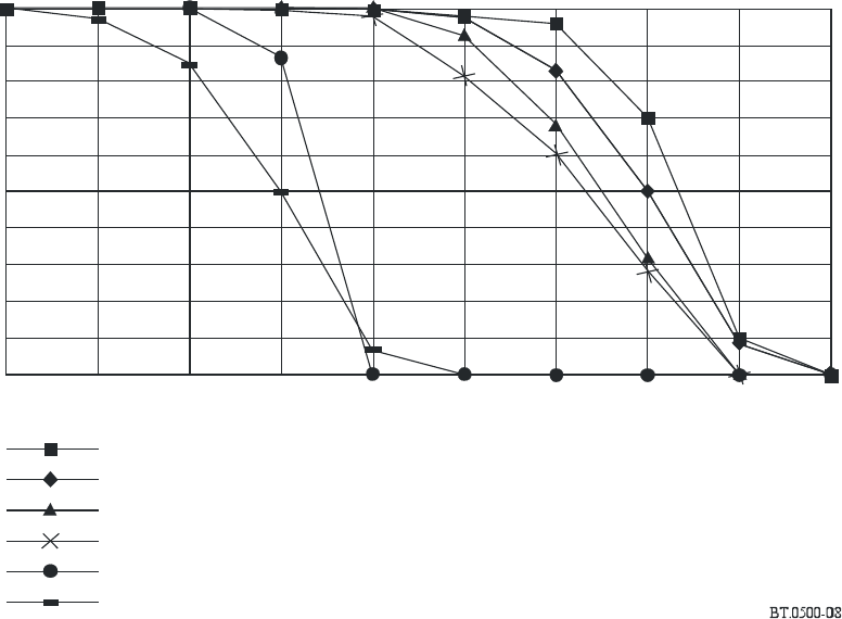
This data can be converted to a histogram of probability, P(q), of the occurrence of quality level q
(see example in Fig. 8).
6.3.2 Calibration of continuous quality results and derivation of a single quality rating
Whilst it has been shown that memory-based biases can exist in longer single rating DSCQS
sessions of digitally-coded video, it has recently been verified that such effects are not significant in
DSCQS assessments of 10 s video excerpts. Consequently, a possible second stage in the SSCQE
process, currently under study, would be to calibrate the quality histogram using the existing
DSCQS method on representative 10 s samples extracted from the histogram data.
Conventional ITU-R methodologies employed in the past have been able to produce single quality
ratings for television sequences. Experiments have been performed which have examined the
relationship between the continuous assessment of a coded video sequence, and an overall single
quality rating of the same segment. It has already been identified that the human memory effects
can distort quality ratings if noticeable impairments occur in approximately the last 10-15 s of the
sequence. However, it has also been found that this human memory effects could be modelled as a
decaying exponential weighting function. Hence a possible third stage in the SSCQE methodology
would be to process these continuous quality assessments, in order to obtain an equivalent single
quality measurement. This is currently under study.
Rec. ITU-R BT.500-13 23
FIGURE 8
Mean of scores of voting sequences on programme segment Z
0
10
20
30
40
50
60
70
80
90
100
0 102030405060708090
Source
Codec W
Analogue 1
Codex X
Analogue 2
Codex Y
P
e
r
c
e
n
t
ag
e
6.4 Simultaneous double stimulus for continuous evaluation (SDSCE) method
The idea of a continuous evaluation came to ITU-R because the previous methods presented some
inadequacies to the video quality measurement of digital compression schemes. The main
drawbacks of the previous standardized methods are linked to the occurrence of context-related
artefacts in the displayed digital images. In the previous protocols, the viewing time duration of
video sequences under evaluation is generally limited to 10 s which is obviously not enough for the
observer to have a representative judgement of what could happen in the real service. Digital
artefacts are strongly dependant upon the spatial and temporal content of the source image. This is
true for the compression schemes but also concerning the error resilience behaviour of digital
transmission systems. With the previous standardized methods it was very difficult to choose
representative video sequences, or at least to evaluate their representativeness. For this reason
ITU-R introduced the SSCQE method, that is able to measure video quality on longer sequences,
representative of video contents and error statistics. In order to reproduce viewing conditions that
are as close as possible to real situations, no references are used in SSCQE.
When fidelity has to be evaluated, reference conditions must be introduced. SDSCE has been
developed starting from the SSCQE, by making slight deviations concerning the way of presenting
the images to the subjects and concerning the rating scale. The method was proposed to MPEG to
evaluate error robustness at very low bit rate, but it can be suitably applied to all those cases where
fidelity of visual information affected by time-varying degradation has to be evaluated.
As a result, the following new SDSCE technique has been developed and tested.
6.4.1 The test procedure
The panel of subjects is watching two sequences in the same time: one is the reference, the other
one is the test condition. If the format of the sequences is SIF (standard image format) or smaller,
the two sequences can be displayed side by side on the same monitor, otherwise two aligned
monitors should be used (see Fig. 9).

24 Rec. ITU-R BT.500-13
FIGURE 9
Example of display format
With error
Reference
Test
condition
Error free
Subjects are requested to check the differences between the two sequences and to judge the fidelity
of the video information by moving the slider of a handset-voting device. When the fidelity is
perfect, the slider should be at the top of the scale range (coded 100), when the fidelity is null, the
slider should be at the bottom of the scale (coded 0).
Subjects are aware of which is the reference and they are requested to express their opinion, while
they are viewing the sequences, throughout their whole duration.
6.4.2 The different phases
The training phase is a crucial part of this test method, since subjects could misunderstand their
task. Written instructions should be provided to be sure that all the subjects receive exactly the same
information. The instructions should include explanation about what the subjects are going to see,
what they have to evaluate (i.e. difference in quality) and how they express their opinion. Any
question from the subjects should be answered in order to avoid as much as possible any opinion
bias from the test administrator.
After the instructions, a demonstration session should be run. In this way subjects are made
acquainted both with voting procedures and kind of impairments.
Finally, a mock test should be run, where a number of representative conditions are shown. The
sequences should be different from those used in the test and they should be played one after the
other without any interruption.
When the mock test is finished, the experimenter should mainly check that in the case of test
conditions equal to the references, the evaluations are close to one hundred (i.e. no difference has
been seen); if instead the subjects declare to see some differences the experimenter should repeat
both the explanation and the mock test.
6.4.3 Test protocol features
The following definitions apply to the test protocol description:
– Video segment (VS): A VS corresponds to one video sequence.
– Test condition (TC): A TC may be either a specific video process, a transmission condition
or both. Each VS should be processed according to at least one TC. In addition, references
should be added to the list of TCs, in order to make reference/reference pairs to be
evaluated.
Rec. ITU-R BT.500-13 25
– Session (S): A session is a series of different pairs VS/TC without separation and arranged
in a pseudo-random order. Each session contains all the VS and TC at least once but not
necessarily all the VS/TC combinations.
– Test presentation (TP): A test presentation is a series of sessions to encompass all the
combinations of VS/TC. All the combinations of VS/TC must be voted by the same number
of observers (but not necessarily the same observers).
– Voting period: Each observer is asked to vote continuously during a session.
– Segment Of Votes (SOV): A segment of 10 s of votes; all the SOV are obtained using
groups of 20 consecutive votes (equivalent to 10 s) without any overlapping.
6.4.4 Data processing
Once a test has been carried out, one (or more) data file is (are) available containing all the votes of
the different sessions (S) representing the total number of votes for the TP. A first check of data
validity can be done by verifying that each VS/TC pair has been addressed and that an equivalent
number of votes has been allocated to each of them.
Data, collected from tests carried out according to this protocol, can be processed in three different
ways:
– statistical analysis of each separate VS;
– statistical analysis of each separate TC;
– overall statistical analysis of all the pairs VS/TC.
A multi-step analysis is required in each case:
– Means and standard deviations are calculated for each vote by accumulation of the
observers.
– Means and standard deviation are calculated for each SOV, as illustrated in Fig. 10. The
results of this step can be represented in a temporal diagram, as shown in Fig. 11.
– Statistical distribution of the means calculated at the previous step (i.e. corresponding to
each SOV), and their frequency of appearance are analysed. In order to avoid the recency
effect due to the previous VS × TC combination, the first 10 SOVs for each VS × TC
sample are rejected.
– The global annoyance characteristic is calculated by accumulating the frequencies of
occurrence. The confidence intervals should be taken into account in this calculation, as
shown in Fig. 12. A global annoyance characteristic corresponds to this cumulative
statistical distribution function by showing the relationship between the means for each
voting segment and their cumulative frequency of appearance.

26 Rec. ITU-R BT.500-13
FIGURE 10
Data processing
1 s
M
SD
1
1
M
SD
2
2
M
SD
v
v
V
20
v
n
, 20
v
1,20
v
1,1
v
2,1
v
n
,1
V
1
sd
1
sd
20
+
+
+
Rejection of the
10 first seconds
Observer 1
Observer 2
Observer (at least 8)
n
Mean: M
i
Standard deviation: SD
i
At least 2 min for 1 combination VS
i
×
TC
k
a) Computation of the mean score, V, and the standard deviation, SD, per instant of vote over the ob servers
for every voting sequence of each combination VS TC×
b) Computation of M and SD per voting sequence of 1 s for each combination VS TC
×
6.4.5 Reliability of the subjects
The reliability of the subjects can be qualitatively evaluated by checking their behaviour when
reference/reference pairs are shown. In these cases, subjects are expected to give evaluations very
close to 100. This proves that at least they understood their task and they are not giving random
votes.
In addition, the reliability of the subjects can be checked by using procedures that are close to that
described in § 2.3.2 of Annex 2 for the SSCQE method.
In the SDSCE procedure, reliability of votes depends upon the following two parameters:
Systematic shifts: During a test, a viewer may be too optimistic or too pessimistic, or may even
have misunderstood the voting procedures (e.g. meaning of the voting scale). This can lead to a
series of votes systematically more or less shifted from the average series, if not completely out of
range.
Local inversions: As in other well-known test procedures, observers can sometimes vote without
taking too much care in watching and tracking the quality of the sequence displayed. In this case,
the overall vote curve can be relatively within the average range. But local inversions can
nevertheless be observed.
These two undesirable effects (atypical behaviour and inversions) could be avoided. Training of the
participants is of course very important. But the use of a tool allowing to detect and, if necessary,
discard inconsistent observers should be possible. A proposal for a two-step process allowing such a
filtering is described in this Recommendation.

Rec. ITU-R BT.500-13 27
FIGURE 11
Raw temporal diagram
01:15:10:12
01:15:27:12
01:15:44:12
01:16:01:12
01:16:18:12
01:16:35:12
01:16:52:12
01:17:09:12
01:17:26:12
01:17:43:12
01:17:43:12
100
90
80
70
60
50
40
30
20
10
0
Time code
Mean
Standard deviation
S
co
r
e
FIGURE 12
Global annoyance characteristics calculated from the statistical
distributions and including confidence interval
10
0
90
80
70
60
50
40
30
20
10
0
0 5 10 15 20 25 30 35 40 45 50 55 60 65 70 75 80 85 90 95
Mean of scores of voting sequences
Critical
No error
Typical
P
e
r
c
e
ntag
e
28 Rec. ITU-R BT.500-13
6.5 Remarks
Other techniques, like multidimensional scaling methods and multivariate methods, are described in
Report ITU-R BT.1082, and are still under study.
All of the methods described so far have strengths and limitations and it is not yet possible to
definitively recommend one over the others. Thus, it remains at the discretion of the researcher to
select the methods most appropriate to the circumstances at hand.
The limitations of the various methods suggest that it may be unwise to place too much weight on a
single method. Thus, it may be appropriate to consider more “complete” approaches such as either
the use of several methods or the use of the multidimensional approach.
Appendix 1
to Annex 1
Picture-content failure characteristics
1 Introduction
Following its implementation, a system will be subjected to a potentially broad range of programme
material, some of which it may be unable to accommodate without loss in quality. In considering
the suitability of the system, it is necessary to know both the proportion of programme material that
will prove critical for the system and the loss in quality to be expected in such cases. In effect, what
is required is a picture-content failure characteristic for the system under consideration.
Such a failure characteristic is particularly important for systems whose performance may not
degrade uniformly as material becomes increasingly critical. For example, certain digital and
adaptive systems may maintain high quality over a large range of programme material, but degrade
outside this range.
2 Deriving the failure characteristic
Conceptually, a picture-content characteristic establishes the proportion of the material likely to be
encountered in the long run for which the system will achieve particular levels of quality. This is
illustrated in Fig. 13.
A picture-content failure characteristic may be derived in four steps:
– Step 1: involves the determination of an algorithmic measure of “criticality” which should
be capable of ranking a number of image sequences, which have been subjected to
distortion from the system or class of systems concerned, in such a way that the rank order
corresponds to that which would be obtained had human observers performed the task. This
criticality measure may involve aspects of visual modelling.
– Step 2: involves the derivation, by applying the criticality measure to a large number of
samples taken from typical television programmes, of a distribution that estimates the
probability of occurrence of material which provides different levels of criticality for the
system, or class of systems, under consideration. An example of such a distribution is
illustrated in Fig. 14.

Rec. ITU-R BT.500-13 29
– Step 3: involves the derivation, by empirical means, of the ability of the system to maintain
quality as the level of criticality of programme material is increased. In practice, this
requires subjective assessment of the quality achieved by the system with material selected
to sample the range of criticality identified in Step 2. This results in a function relating the
quality achieved by the system to the level of criticality in programme material. An
example of such a function is given in Fig. 15.
– Step 4: involves the combination of information from Steps 2 and 3 in order to derive a
picture-content failure characteristic of the form given in Fig. 13.
FIGURE 13
Graphical representation of possible picture content
failure characteristic
High
Low
High
Low
Picture quality
P
r
o
b
a
b
i
l
i
t
y
(
i.
e
.
,
p
r
o
p
o
r
t
i
o
n
of typical programme material)
FIGURE 14
Probability of occurrence of material of differing
levels of criticality
P
r
obabi
l
it
y
(i.
e
.
,
p
r
opo
r
tion
of typical programme material)
High
Low
High
Index of criticality
Low
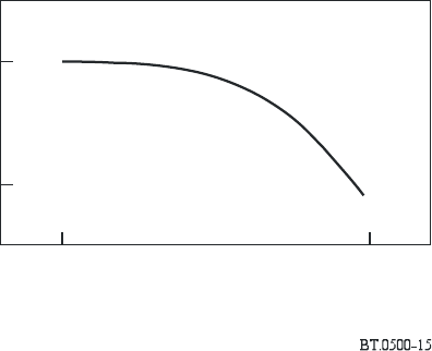
30 Rec. ITU-R BT.500-13
FIGURE 15
A possible function relating quality to the criticality
of programme material
Index of criticality
Q
ua
l
it
y
High
Low
High
Low
3 Use of the failure characteristic
In providing an overall picture of the performance likely to be achieved over the range of possible
programme material, the failure characteristic is an important tool for considering the suitability of
systems. The failure characteristic can be used in three ways:
– to optimize parameters (e.g. source resolution, bit rate, bandwidth) of a system at the design
stage to match it more closely to the requirements of a service;
– to consider the suitability of a single system (i.e. to anticipate the incidence and severity of
failure during operation);
– to assess the relative suitabilities of alternative systems (i.e. to compare failure
characteristics and determine which system would be more suitable for use). It should be
noted that, while alternative systems of a similar type may use the same index of criticality,
it is possible that systems of a dissimilar type may have different indices of criticality.
However, as the failure characteristic expresses only the probability that different levels of
quality will be seen in practice, characteristics can be compared directly even when derived
from different, system-specific indices of criticality.
While the method described in this Recommendation provides a means of measuring the picture-
content failure characteristic of a system, it may not fully predict the acceptability of the system to
the viewer of a television service. To obtain this information it may be necessary for a number of
viewers to watch programmes encoded with the system of interest, and to examine their comments.
An example of picture-content failure characteristics for digital television is described in Annex 1 to
Recommendation ITU-R BT.1129.
Rec. ITU-R BT.500-13 31
Appendix 2
to Annex 1
Method of determining a composite failure characteristic
for programme content and transmission conditions
1 Introduction
A composite failure characteristic relates perceived image quality to probability of occurrence in
practice in a way that explicitly considers both programme content and transmission conditions.
In principle, such a characteristic could be derived from a subjective study that involves sufficient
numbers of observations, times of test, and reception points to yield a sample that represents the
population of possible programme content and transmission conditions. In practice, however, an
experiment of this sort may be impracticable.
The present Appendix describes an alternative, more readily realized procedure for determining
composite failure characteristics. This method consists of three stages:
– programme-content analysis;
– transmission-channel analysis;
– derivation of composite failure characteristics.
2 Programme-content analysis
This stage involves two operations. First, an appropriate measure of programme content is derived
and, second, the probabilities with which values of this measure occur in practice are estimated.
A programme-content measure is a statistic that captures aspects of programme content that stress
the ability of the system(s) under consideration to provide perceptually faithful reproductions of
programme material. Clearly, it would be advantageous if this measure were based on an
appropriate perceptual model. However, in the absence of such a model, a measure that captures
some aspect of the extent of spatial diversity within and across video frames/fields might suffice,
provided this measure enjoys a roughly monotonic relation with perceived image quality. It may be
necessary to use different measures for systems (or classes of systems) that use fundamentally
different approaches to image representation.
Once an appropriate measure has been selected, it is necessary to estimate the probabilities with
which the possible values of this statistic occur. This can be done in one of two ways:
– with the empirical procedure, a random sample of perhaps 200 10 s programme segments in
a studio format suited in resolution, frame rate, and aspect ratio to the system(s) considered
is analysed. Analysis of this sample yields relative frequencies of occurrence for values of
the statistic which are taken as estimates of probability of occurrence in practice; or
– with the theoretical method, a theoretical model is used to estimate the probabilities. It
should be noted that, although the empirical method is preferred, it may be necessary in
specific cases to use the theoretical method (e.g. when there is not sufficient information
about programme content, such as with the emergence of new production technologies).
The foregoing analyses will result in a probability distribution for values of the content statistic (see
also Appendix 1 to Annex 1). This will be combined with the results of the transmission-conditions
analysis to prepare for the final stage of the process.
32 Rec. ITU-R BT.500-13
3 Transmission-channel analysis
This stage also involves two operations. First, a measure of transmission-channel performance is
derived. And, second, the probabilities with which values of this measure occur in practice are
estimated.
A transmission-channel measure is a statistic that captures aspects of channel performance that
influence the ability of the system(s) under consideration to provide perceptually faithful
reproductions of source material. Clearly, it would be advantageous if this measure were based on
an appropriate perceptual model. However, in the absence of such a model, a measure that captures
some aspect of the stress imposed by the channel might suffice, provided this measure enjoys a
roughly monotonic relation with perceived image quality. It may be necessary to use different
measures for systems (or classes of systems) that use fundamentally different approaches to channel
coding.
Once an appropriate measure has been selected, it is necessary to estimate the probabilities with
which the possible values of this statistic occur. This can be done in one of two ways:
– with the empirical procedure, channel performance is measured at perhaps 200 randomly
selected times and reception points. Analysis of this sample yields relative frequencies of
occurrence for values of the statistic which are taken as estimates of probability of
occurrence in practice; or
– with the theoretical method, a theoretical model is used to estimate the probabilities. It
should be noted that, although the empirical method is preferred, it may be necessary in
specific cases to use the theoretical method (e.g. when there is not sufficient relevant
information about channel performance, such as with the emergence of new transmission
technologies).
The foregoing analyses will result in a probability distribution for values of the channel statistic.
This will be combined with the results of the programme-content analysis to prepare for the final
stage of the process.
4 Derivation of composite failure characteristics
This stage involves a subjective experiment in which programme content and transmission
conditions are varied jointly according to probabilities established in the first two stages.
The basic method used is the double-stimulus continuous quality procedure and, in particular, the
10 s version recommended for motion sequences (see Annex 1, § 5). Here, the reference is a picture
at studio quality in an appropriate format (e.g. one with resolution, a frame rate, and an aspect ratio
appropriate to the system(s) considered). In contrast, the test presents the same picture as it would
be received in the system(s) considered under selected channel conditions.
Test material and channel conditions are selected in accordance with probabilities established in the
first two stages of the method. Segments of test material, each of which has been analysed to
determine its predominant value according to the content statistic, comprise a selection pool.
Material is then sampled from this pool such that it covers the range of possible values of the
statistic, sparsely at less critical levels and more densely at more critical levels. Possible values of
the channel statistic are selected in a similar way. Then, these two independent sources of influence
are combined randomly to yield combined content and channel conditions of known probability.
The results of such studies, which relate perceived image quality to probability of occurrence in
practice, are then used to consider the suitability of a system or to compare systems in terms of
suitability.
Rec. ITU-R BT.500-13 33
Appendix 3
to Annex 1
Contextual effect
Contextual effects occur when the subjective rating of an image is influenced by the order and
severity of impairments presented. For example, if a strongly impaired image is presented after a
string of weakly impaired images, viewers may inadvertently rate this image lower than they
normally might have.
A group of four laboratories in different countries investigated possible contextual effects
associated with the results of three methods (DSCQS method, DSIS method variant II and a
comparison method) used to evaluate picture quality. Test material was produced using MPEG
(ML@MP) coding along with reduction of horizontal resolution. Four basic test conditions (B1, B2,
B3, B4) along with six contextual test conditions were applied to each test series, one depicting
weak contextual impairments and the other depicting strong impairments. The three test methods
were applied to both test series. Contextual effects are the difference between the results for the test
containing predominantly weak impairments and the test containing predominantly strong
impairments. The basic test conditions B2 and B3 were used to determine contextual effects.
Results of the combined laboratories indicate no contextual effects for the DSCQS method. For the
DSIS and comparison methods contextual effects were evident and the strongest effect was found
for the DSIS method variant II. Results indicate that predominantly weak impairments can cause
lower ratings for an image whereas predominantly strong impairments can cause higher ratings.
Results of the investigation suggest that the DSCQS method is the better method to minimize
contextual effects for subjective picture quality assessment recommended by ITU-R.
More information about the investigation mentioned above is given in Report ITU-R BT.1082.
Annex 2
Analysis and presentation of results
1 Introduction
In the course of a subjective experiment to assess the performance of a television system, a large
amount of data is collected. These data, in the form of observers’ score sheets, or their electronic
equivalent, must be condensed by statistical techniques to yield results in graphical and/or
numerical/formulae/algorithm form which summarize the performance of the systems under test.
The following analysis is applicable to the results of SS methods, the DSIS method, and the
DSCQS method for the assessment of television picture quality which are found in this
Recommendation (§ 4, 5 and 6 in Annex 1) and to other alternative methods using numerical scales.
In the first and the second case, the impairment is rated on a five-point or multi-point scale. In the
last case, continuous rating scales are used and the results (differences of the ratings for the
reference picture and the actual picture under test) are normalized to integer values between
0 and 100.

34 Rec. ITU-R BT.500-13
2 Common methods of analysis
Tests performed according to the principles of methods described in Annex 1 will produce
distributions of integer values e.g. between 1 and 5 or between 0 and 100. There will be variations
in these distributions due to the differences in judgement between observers and the effect of a
variety of conditions associated with the experiment, for example, the use of several pictures or
sequences.
A test will consist of a number of presentations, L. Each presentation will be one of a number of test
conditions, J applied to one of a number of test sequences/test images, K. In some cases each
combination of test sequence/test image and test condition may be repeated a number of times, R.
2.1 Calculation of mean scores
The first step of the analysis of the results is the calculation of the mean score,
,
jkr
u
for each of the
presentations:
=
=
N
i
ijkr
u
N
jkr
u
1
1
(1)
where:
u
ijkr
: score of observer i for test condition j, sequence/image k, repetition r
N: number of observers.
Similarly, overall mean scores,
j
u
and ,
k
u could be calculated for each test condition and each test
sequence/image.
2.2 Calculation of confidence interval
2.2.1 Processing of raw (uncompensated and/or unapproximated) data
When presenting the results of a test all mean scores should have an associated confidence interval
which is derived from the standard deviation and size of each sample.
It is proposed to use the 95% confidence interval which is given by:
[]
jkrjkrjkrjkr
u,u δδ +−
where:
N
S
jkr
jkr
96.1=δ
(2)
The standard deviation for each presentation, S
jkr
, is given by:
=
−
−
=
N
i
ijkrjkr
jkr
N
uu
S
1
2
)1(
)(
(3)
With a probability of 95%, the absolute value of the difference between the experimental mean
score and the “true” mean score (for a very high number of observers) is smaller than the 95%
confidence interval, on condition that the distribution of the individual scores meets certain
requirements.

Rec. ITU-R BT.500-13 35
Similarly, a standard deviation S
j
could be calculated for each test condition. It is noted however
that this standard deviation will, in cases where a small number of test sequences/test images are
used, be influenced more by differences between the test sequences used than by variations between
the assessors participating in the assessment.
2.2.2 Processing of compensated and/or approximated data
For data for which the evaluation scale residual impairment/enhancement and boundary effects have
been compensated, or data presented in the form of an impairment response or impairments addition
law after approximation, (due to the dependence of experimental quality mean scores to these
distortions), the confidence interval should be calculated using statistical variable transformations
taking into account the dispersion of the according variable.
If quality assessment results are presented as an impairment response (i.e. experimental curve), the
lower and upper confidence limits of the confidence interval will be the function of each
experimental value. To calculate these confidence limits the standard deviation has to be calculated
and an approximation of its dependence has to be evaluated for each experimental value of the
original impairment response.
2.3 Screening of the observers
2.3.1 Screening for DSIS, DSCQS and alternative methods except SSCQE method
First, it must be ascertained whether this distribution of scores for test presentation is normal or not
using the β
2
test (by calculating the kurtosis coefficient of the function, i.e. the ratio of the fourth
order moment to the square of the second order moment). If β
2
is between 2 and 4, the distribution
may be taken to be normal. For each presentation the scores u
ijkr
of each observer must be
compared with the associated mean value,
,
jkr
u
plus the associated standard deviation, S
jkr
, times
two (if normal) or times
20 (if non-normal), P
jkr
, and to the associated mean value minus the
same standard deviation times two or times
,20
Q
jkr
. Every time an observer’s score is found
above P
jkr
a counter associated with each observer, P
i
, is incremented. Similarly, every time an
observer’s score is found below Q
jkr
a counter associated with each observer, Q
i
, is incremented.
Finally, the following two ratios must be calculated: P
i
+ Q
i
divided by the total number of scores
from each observer for the whole session, and P
i
– Q
i
divided by P
i
+ Q
i
as an absolute value. If the
first ratio is greater than 5% and the second ratio is less than 30%, then observer i must be
eliminated (see Note 1).
NOTE 1 – This procedure should not be applied more than once to the results of a given experiment.
Moreover, use of the procedure should be restricted to cases in which there are relatively few observers
(e.g. fewer than 20), all of whom are non-experts.
This procedure is recommended for the EBU method (DSIS); it has also been successfully applied
to the DSCQS method and alternative methods.
The above process can be expressed mathematically as:
For each test presentation, calculate the mean,
,
jkr
u
standard deviation, S
jkr
, and kurtosis
coefficient, β
2jkr
, where β
2jkr
is given by:
2
2
4
2
)(m
m
jkr
=β with
N
u
u
m
N
i
x
ijkrijkr
x
=
=
1
)
–
(
(4)
For each observer, i, find P
i
and Q
i
, i.e.:
for j, k, r = 1, 1, 1 to J, K, R

36 Rec. ITU-R BT.500-13
if 2 ≤ β
2jkr
≤ 4, then:
if
jkrjkr
ijkr
Suu 2+≥
then P
i
= P
i
+ 1
if
jkrjkr
ijkr
Suu 2–≤
then Q
i
= Q
i
+ 1
else:
if
jkrjkr
ijkr
Suu 20+≥
then P
i
= P
i
+ 1
if
jkrjkr
ijkr
Suu 20–≤
then Q
i
= Q
i
+ 1
If
R
K
J
QP
ii
⋅⋅
+
> 0.05 and
ii
ii
QP
QP
+
−
< 0.3 then reject observer i
with:
N
: number of observers
J
: number of test conditions including the reference
K
: number of test pictures or sequences
R
: number of repetitions
L
: number of test presentations (in most cases the number of presentations will be
equal to J
· K · R, however it is noted that some assessments may be conducted
with unequal numbers of sequences for each test condition).
2.3.2 Screening for SSCQE method
For specific observer screening when using the SSCQE test procedure, the application domain is
not anymore one of the test configurations (combination of a test condition and a test sequence) but
a time window (e.g. 10 s vote segment) of a test configuration. There is a two step filtering, the first
one is devoted to detection and discarding of observers exhibiting a strong shift of votes compared
to the average behaviour, the second one is made for detection and screening of inconsistent
observers without any consideration of systematic shift.
Step 1: Detection of local vote inversions
Here also, it must be first ascertained whether this distribution of scores for each time window of
each test configuration is “normal”, or not, using the β
2
test. If β
2
is between 2 and 4, the
distribution may be considered as “normal”. Then, the process applies for each time window of
each test configuration as mathematically expressed hereafter.
For each time window of each test configuration and using the votes u
ijkr
of each observer, the
mean,
,
jklr
u
standard deviation, S
jklr
, and the coefficient, β
2jklr
, are calculated. β
2jklr
is given by:
2
2
4
2
)(
β
m
m
jklr
= with
N
u
u
m
N
n
x
njklr
x
=
−
=
1
)(
For each observer, i, find P
i
and Q
i
, i.e.:
for j, k, l, r = 1, 1, 1, 1 to J, K, L, R
if 2 ≤ β
2jklr
≤ 4, then:
if
jklr
jklrnjklr
Suu 2+≥
then P
i
= P
i
+ 1
if
jklr
jklrnjklr
Suu 2+≤
then Q
i
= Q
i
+ 1

Rec. ITU-R BT.500-13 37
else:
if
jklr
jklrnjklr
Suu 20+≥
then P
i
= P
i
+ 1
if
jklr
jklrnjklr
Suu 20–≤
then Q
i
= Q
i
+ 1
If
R
L
K
J
P
i
⋅⋅⋅
> X% or
R
L
K
J
Q
i
⋅⋅⋅
> X% then reject observer i
with:
N
: number of observers
J
: number of time windows within a test combination of test condition and
sequence
K
: number of test conditions
L
: number of sequences
R
: number of repetitions.
This process allows to discard observers who have produced votes significantly distant from the
average scores. Figure 17 shows two examples (the two extreme curves exhibiting important shifts).
Nevertheless, this rejection criteria does not allow to detect possible inversions which is another
important source of bias. For that reason a second process step is proposed.
Step 2: Detection of local vote inversions
For Step 2, the detection is also based on the screening formulae given in Annex 2 of the present
Recommendation. A slight modification concerning the application domain is introduced. The input
data set is again constituted by the scores of all the time windows (e.g. 10 s) of all the test
configurations. But this time the scores are preliminary centred around the overall mean to
minimize the shift effect which has been already been treated at the first process stage. The usual
process is then applied.
It must be first ascertained whether this distribution of scores for each time window of each test
configuration is “normal”, or not, using the β
2
test. If β
2
is between 2 and 4, the distribution may be
taken as “normal”. Then, the process applies for each time window of each test configuration as
mathematically expressed hereafter.
The first step of the process is the calculation of centred scores for each time window and each
observer. The mean score,
,
klr
u
for each of the test configuration being defined as:
==
⋅=
N
n
J
j
njklrklr
u
JN
u
11
11
Similarly the mean score for each test configuration and each observer is defined as:
=
=
J
j
njklrnklr
u
J
u
1
1
and u
njklr
corresponds to the score of observer i for time window j, test condition k, sequence l,
repetition r.
For each observer, the centred scores u
*
njklr
are calculated as follows:
klrnklrnjklr
njklr
uuuu +−=*

38 Rec. ITU-R BT.500-13
For each time window of each test configuration, the mean,
,*
jklr
u
the standard deviation, S *
jklr
,
and the coefficient, β
2
∗
jklr
, are calculated. β
2
∗
jklr
, is given by:
2
2
4
*
2
)(m
m
jklr
=β with
N
u
m
N
n
x
njklr
x
=
=
1
*
)(
For each observer, i, find P*
i
and Q*
i
, i.e.:
for j, k, l, r = 1, 1, 1, 1 to J, K, L, R
if 2 ≤ β
2
*
jklr
≤ 4, then:
if
jklr
jklr
njklr
Suu *2** +≥ then P*
i
= P*
i
+ 1
if
jklr
jklr
njklr
Suu *2** –≤ then Q*
i
= Q*
i
+ 1
else:
if
jklr
jklr
njklr
Suu *20** +≥ then P*
i
= P*
i
+ 1
if
jklr
jklr
njklr
Suu *20–** ≤ then Q*
i
= Q*
i
+ 1
If
R
L
K
J
QP
ii
⋅⋅⋅
+
**
> Y and
ii
ii
QP
QP
**
**
+
−
< Z then reject observer i
with:
N
: number of observers
J
: number of time windows within a test combination of test condition and
sequence
K
: number of test conditions
L
: number of sequences
R
: number of repetitions.
Proposed values for parameters (X, Y, Z) experienced as adapted to this method are 0.2, 0.1, 0.3.
3 Processing to find a relationship between the mean score and the objective measure of
a picture distortion
If subjective tests were carried out in order to investigate the relation between the objective measure
of a distortion and the mean scores
u
(
u
calculated according to § 2.1), the following process can
be useful, which consists of finding a simple continuous relationship between
u
and the
impairment parameter.
3.1 Approximation by a symmetrical logistic function
The approximation of this experimental relationship by a logistic function is particularly interesting.
The processing of the data
u
can be made as follows:
The scale of values
u
is normalized by taking a continuous variable p so that,
p = (
u – u
min
) / (u
max
– u
min
) (5)

Rec. ITU-R BT.500-13 39
with:
u
min :
minimum score available on the u-scale for the worst quality
u
max
: maximum score available on the u-scale for the best quality.
Graphical representation of the relationship between p and D shows that the curve tends to be a
skew-symmetrical sigmoid shape provided that the natural limits to the values of D extend far
enough from the region in which u varies rapidly.
The function p = f (D) can now be approximated by a judiciously chosen logistic function, as given
by the general relation:
p = 1
/ [1 + exp ( D – D
M
) G ] (6)
where D
M
and G are constants and G may be positive or negative.
The value p obtained from the optimum logistic function approximation is used to provide a
deduced numerical value I according to the relation:
I = (1/p – 1) (7)
The values of D
M
and G can be derived from the experimental data after the following
transformation:
I = exp (
D – D
M
) G (8)
This yields a linear relation by the use of a logarithmic scale for I:
log
e
I = ( D – D
M
) G (9)
Interpolation by a straight line is simple and in some cases of an accuracy which is sufficient for the
straight line to be considered as representing the impairment due to the effect measured by D.
The slope of the characteristic is then expressed by:
GI
DD
S
M
1
log
e
=
−
=
(10)
which yields the optimum value of G. D
M
is the value of D for I = 1.
The straight line may be termed the impairment characteristic associated with the particular
impairment being considered. It will be noted that the straight line can be defined by the
characteristic values D
M
and G of the logistic function.
3.2 Approximation by a non-symmetrical function
3.2.1 Description of the function
The approximation of the relationship between the experimental scores and the objective measure
of a picture distortion by a symmetrical logistic function is mostly successful in the case that the
distortion parameter D can be measured in a related unit, e.g. the S/N (dB). If the distortion
parameter was measured in a physical unit d, e.g. a time delay (ms), the relation (8) has to be
replaced by:
I = (
d / d
M
)
1/G
(11)
and therefore (6) becomes:
[]
G/1
)/(11
M
ddp += (12)
This function approximates the logistic one in a non-symmetrical way.

40 Rec. ITU-R BT.500-13
3.2.2 Estimation of the parameters of the approximation
The estimation of the optimal parameters of the function that provides the minimum residual errors
between the actual data and the function may be obtained with any recursive estimation algorithm.
Figure 16 shows an example of the use of the non-symmetrical function to represent actual
subjective data. This representation allows the estimation of specific objective measures
corresponding to interesting subjective value: 4.5 on the five-grade scale, for instance.
FIGURE 16
Non-symmetrical approximation
0
1
2
3
4
5
pd
()
d
3.3 Correction of the residual impairment/enhancement and the scale boundary effect
In practice, the use of a logistic function sometimes cannot avoid some differences between
experimental data and approximation. These discrepancies may be due to the end of scale effects or
simultaneous presence of several impairments in the test which may influence the statistical model
and deform the theoretical logistic function.
A kind of scale boundary effect has been identified in which observers tend not to use the extreme
values of the judgement scale, in particular for high quality scores. This may arise from a number of
factors, including a psychological reluctance to make extreme judgements. Moreover the use of the
arithmetical mean of judgements according to equation (1) near the scale boundaries may cause
biased results because of the non-Gaussian distribution of votes in these areas.
Frequently a residual impairment (even in reference pictures the mean score only reaches a value
)
0 max
uu < is stated in the tests.
There are some useful approaches to correct the raw data of assessments for processing valid
conclusions (see Table 5).
The correction of boundary effects if they exist in experimental data is a part of data processing of
great importance. So, choice of procedure must be done with great accuracy. Note that these
correction procedures involve special assumptions, so caution is advised in using them; their use
should be reported in the presentation of the results.

Rec. ITU-R BT.500-13 41
TABLE 5
Comparison of methods of correction of the scale boundary effects
3.4 Incorporation of the reliability aspect in the graphs
From the mean grades for each impairment tested and the associated 95% confidence intervals,
three series of grades are constructed:
– minimum grade series (means – confidence intervals);
– mean grade series;
– maximum grade series (means + confidence intervals).
The estimation parameters for the three series are then estimated independently. The three functions
obtained can then be drawn on the same graph, the two from the maximum and minimum series as
dotted lines and the mean estimate as a solid line. The experimental values are also plotted on this
graph (see Fig. 17). We thus get an estimate of the 95% continuous confidence region.
For the grade 4.5 (threshold of visibility for the method) we can thus read off directly from the
graph an estimated 95% confidence interval that can be used to determine a tolerance range.
The space between the maximum and minimum curves is not a 95% interval, but a mean estimate
thereof.
At least 95% of the experimental values should lie within the confidential region; otherwise it may
be concluded that there was a problem in carrying out the test or that the function model chosen was
not the optimum one.
Boundary effects
compensation methods
Features
Residual impairment
compensation
Residual enhancement
compensation
Shift in the centre
of the scale
No compensation No No No
Linear scale transformation Yes May be significant error No
Non-linear scale transformation
(1)
Yes Yes No
Imps addition based method Yes No Yes
Multiplicative method Yes No Yes
(1)
According to the non-linear scale transformation the corrected votes have to be calculated:
midmidcorr
uuuCu +−= )(
mid
midmin
mid
midmax
uu
uu
uu
uu
uu
uu
uu
uu
C
min
min
max
max
max
min
max
min
−
−
−
−
+
−
−
−
−
=
000
0
000
0
with:
u
corr
: corrected score
u : uncorrected experimental score
u
min
, u
max
: boundaries of the voting scale
u
mid
: middle of the voting scale
u
0
min
, u
0
max
: lower and upper boundaries of the tendency of experimental scores.

42 Rec. ITU-R BT.500-13
FIGURE 17
Case of non-symmetrical impairment characteristic
pd
()
qd
()
rd
()
0
1
2
3
4
5
d
pd
qd
rd
d
( ): mean grade series
( ): minimum grade series
( ): maximum grade series
: objective impairment measurement
4 Conclusions
A procedure for the evaluation of the confidence intervals, i.e. the accuracy's of a set of subjective
assessment tests, has been described.
The procedure also leads to the estimation of mean general quantities that are relevant not only to
the particular experiment under consideration, but also to other experiments carried out with the
same methodology.
Therefore, such quantities may be used to draw diagrams of the confidence interval behaviour
which are helpful for the subjective assessments, as well as for planning future experiments.
Rec. ITU-R BT.500-13 43
Annex 3
Description of a common inter-change data file format
The purpose of a common inter-change data file format is to facilitate exchange of data between
laboratories taking part in a collaborative international subjective evaluation campaign.
Any subjective evaluation assessment is developed according to five successive and dependent
phases: test preparation, test performing, data processing, results presentation and interpretation. It
is usually the case that, in large international campaigns, the work is distributed between the
different laboratories participating:
– A laboratory has the responsibility to setup the test, in collaboration with other parties, by
identifying the quality parameters to be assessed, the test material to be used (currently
critical but not unduly so), the test framework (e.g. methodology, viewing distances,
session arrangement, sequence of test item presentation) and the test environment (e.g.
viewing conditions, introductory speech).
– Volunteering laboratories are asked to provide the test material processed according to the
appropriate techniques representative of the quality parameter to be assessed (simulation or
hardware based).
– A different partner is responsible for editing the test tape.
– Different volunteering laboratories are performing the test using the preliminary edited
tape. The test can be a blind test. In this case, the laboratory will carry out the test by
gathering the assessors’ votes without necessarily knowing the quality parameters under
evaluation.
– Another participant is generally requested to coordinate the collection of the resulting raw
data for processing and edition of results, which can also be done blindly.
– Finally, the results are interpreted from a text/table or graphic representation, and a final
report is published.
The format proposed allows the gathering of results delivered according to the test procedures
defined during the test definition phase.
The format is compliant with the evaluation methods described in Recommendation ITU-R BT.500.
It is made of text files with a structure which is shown in Tables 6 and 7. Its syntax is built around
labels and fields in addition to a limited set of reserved symbols (e.g. “
[”, “]”, “ ”, “↵” and “=”).
There is no intrinsic limitation in terms of capacity (e.g. the number of participating laboratories,
observers, test sequences and quality parameters, voting scale boundaries or the type of voting
peripheral).

44 Rec. ITU-R BT.500-13
TABLE 6
Identification results text file format
TABLE 7
Results.DAT raw data text file format
Identification file format and syntax Comments
[Test framework]↵
Type = “DSCQS” or “DSIS I”, “DSIS II”, etc.
↵
Number of sessions = 1
≤
integer
≤
x↵
Scale minimum = integer↵
Scale maximum = integer
↵
Monitor size = integer
↵
Monitor make and model = chain of characters↵
[Section identifier]
Identification of Rec. ITU-R BT.500 methodology used
Number of sessions
(1)
in which a test has been distributed
Definition of the scale (see methodology specific requirements,
if any)
Display diagonal (in)
[RESULTS] ↵
Number of results = 1
≤
integer
≤
y↵
Result(j).Filename(s) = character string.DAT
↵
....
Result(j).Name = character string
↵
Result(j).Laboratory = character string
↵
Result(j).Number of observers = 1
≤
integer
≤
N↵
Result(j).Training = “Yes” or “No” ↵
[Section identifier]
Number of Results
(1)
files being considered
Full.DAT (see Table 7) filename including the path
Custom Results file name
Identification of the test performing laboratory
Total number of observers
Indicates if the votes gathered during the training are included
the DAT file attached
[Result(j).Session(i).Observers] ↵
O(k).First Name = character string
↵
O(k).Last Name = character string
↵
O(k).Sex = “F” or “M” ↵
O(k).Age = integer↵
O(k). Occupation = character string
↵
O(k).Distance = integer↵
[Section identifier]
Observer identification
Optional
Optional
Main socio-economic groups (e.g. worker, student)
Viewing distance in display heights (e.g. 3 H, 4 H, 6 H)
(1)
Session: A test can be divided in a number of different sessions to cope with the maximum test duration requirement. The same
or different observers can attend different sessions during which they will be asked to assess different test items. The merging of
votes gathered from different sessions gives a complete set of test results (number of presentations × number of votes per
p
resentation). Results can be attached in different .DAT files which would be delivered for each performance.
filename.DAT File Format and
Syntax
Comments
integer integer integer.......↵
integer integer integer.......↵
integer integer integer.......↵
.....
A DAT raw data file is made of vote values separated by a space. One
line should be used per observer
Raw data is stored in the order of entry
Data can be distributed in different DAT files identified in Table 6 by
Result(j). Filename(s)
(1)
.
(1)
See
(1)
to Table 6.
