Slide 1

Using Excel for Research

Oct 1, 2021

Oregon Health & Science University

Presented by Julie Mitchell - OCTRI Informatics Manger

Agenda

• Recommended uses for Excel

• Challenges with Excel

• Caveats to using Excel

• Techniques for cleaning, validating & transforming data

When should I NOT USE Excel?

• Storing your data

• Data transformation where code can be written, saved, and most

importantly logged to track the changes that were made to the data

• Statistical analysis or calculations

When should I consider using Excel?

• Data exploration

• Error checking

• Data cleaning

• Data validation

• Reformatting datasets for import into a database

Common Data Discrepancies

• More than one item per cell

• Inconsistent units for numbers

• For numbers, number of decimal places inconsistent

• Inconsistent data values in each column

• Date formatting inconsistent

Additional Challenges with Excel

• Missing values are handled inconsistently, and sometimes incorrectly when using formulas.

• Data organization differs according to analysis, forcing you to reorganize your data in many

ways if you want to do many different analyses.

• Many analyses can only be done on one column at a time, making it inconvenient to do the

same analysis on many columns.

• Output is poorly organized, sometimes inadequately labeled, and there is no record of how

an analysis was accomplished.

• Doesn’t allow complex workflows

• Single allow multi-user access at a single time

• Scalability - limited ability to automate tasks

• Security

Caveats to Using Excel

1. Always format your data prior to applying any formulas or clean-

2. Clean only what you cannot clean in your statistical analysis

software

3. BEFORE cleaning or reformatting data rename and save your

spreadsheet

4. ALWAYS duplicate a column before “cleaning or reformatting”

5. AFTER each data cleaning or reformatting step, rename and save

your spreadsheet

6. Establish file format standards

7. Use a standard versioning system

Excel File Types

File Formatting Standards

1. Variable names in columns and observations in rows.

2. Put variable names in the first row.

3. Use a separate column for each piece of information.

4. When entering dates (especially for years prior to 1930) include a 4 digit

year. Don’t calculate date differences in Excel.

5. Decide on "missingness" conventions.

6. Do not "stack" data on the same sheets.

7. Document your data cleaning.

Excel Lingo &

Data Organization

Ensure that the data are in

a tabular format of rows

and columns with:

1) Similar data in each

column

2) All columns and rows

visible

3) No blank rows within

the range

Do tasks that don't require

column manipulation first,

such as spell-checking or

using the Find and

Replace dialog box

Commands

ribbon

Column labels

(A, B, C, D…)

Cell

(I6)

Worksheets

Scroll bars

HINT: If you open a file in excel and you see a column with

##### signs in it, the column is too narrow to display the full

number and you need to adjust the column width.

Row labels

(1, 2, 3, 4…)

Formatting a Cell

Standardize cells in each column

Format cell contents- insert spaces, dashes,

parentheses… (only works with numbers)

1) Select the cells that you want to

format (cell(s) need to be in a number

type format- not general or text)

In Windows version:

2) Click on Home tab

3) Click on Font Settings

In Apple version:

2) Click on Format on top menu bar

3) Click on Cells

------------------------------------------------

4) Click on Number tab in the Format

Cells dialog box

5) Click on Special under Category

6) Select an option (example shows

Phone Number)

Font Settings

Home Tab

Number Tab

Type

Special Category

HINT: Always note which cells contain information that is not

displayed. Use the Wrap-Text option to display the text

Wrap Text

Change cell contents by inserting spaces, dashes,

parentheses.

TIP #1

If you open a file in excel and you see a column with

###### or cells that end with E+09, the column is

too narrow to display the full number and you need

to adjust the column width.

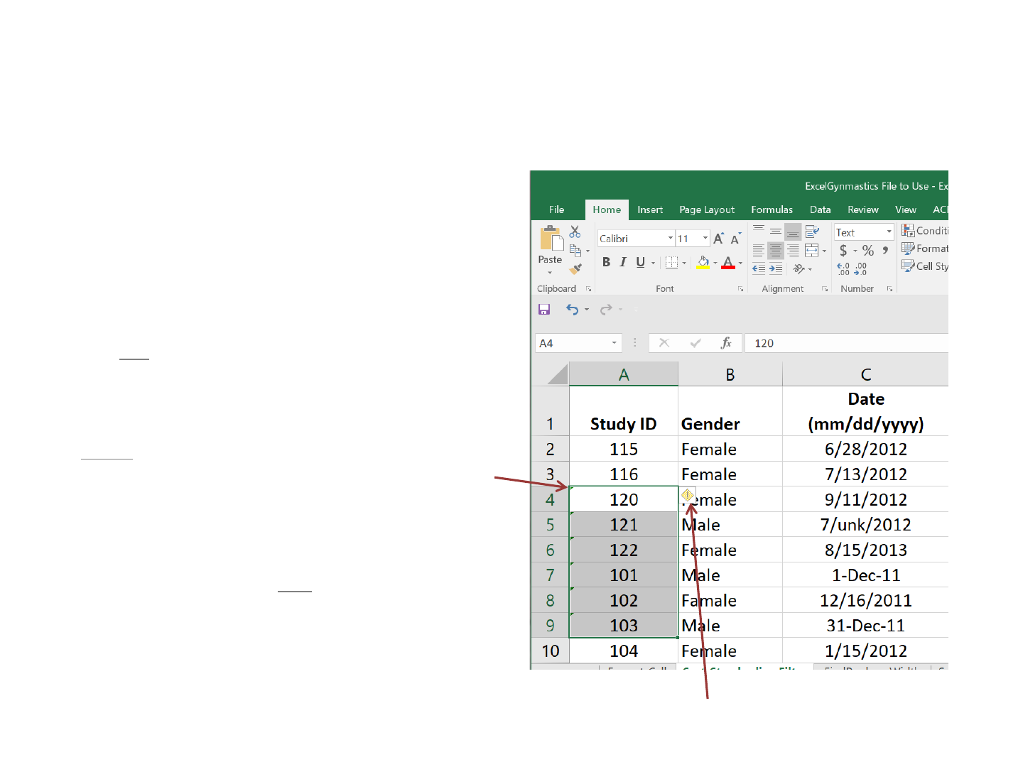
Standardizing Cell

Formats (Part 1 of 2)

There are two main issues with numbers

that may require you to clean the data: the

number was inadvertently imported as text

or the negative sign needs to be changed

1) Select only the cells with errors (green

flag in top left corner). Be careful to

NOT include the header or empty cells

2) Click on error box and then select

Convert to Number

NOTES & WARNINGS:

Do not:

• Try changing the cell format (Number:

Category) Home tab: Font: Number

tab: Category

• Try changing the format using the

quick Number Format

These options only work for NEW data entry.

If cells are already pre-populated and have a

“text” format they will not reformat.

Error

Error Box

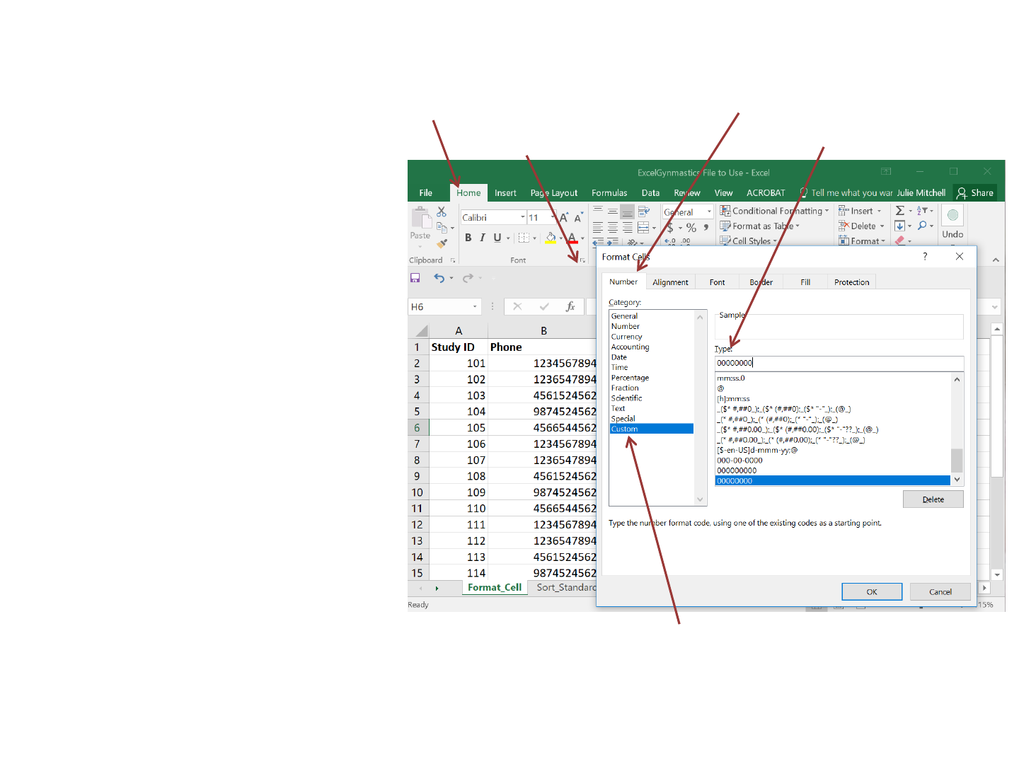
Standardizing Cell

Formats (Part 2 of 2)

Leading Zeros: If you have leading zeros –

which may occur with medical record

numbers, etc. Set the cell format to “Text” or

create a “Custom” format where you can also

specify the character length and format.

How to create a special format:

1) Select the cells that you want to format

(cell(s) need to be in a number type

format- not general or text)

In Windows version:

2) Click on Home tab

3) Click on Font Settings

In Apple version:

2) Click on Format on top menu bar

3) Click on Cells

------------------------------------------------

4) Click on Number tab in the Format Cells

dialog box

5) Click on Custom under Category

6) Type in the format that you want in

Type field

Font Settings

Home Tab

Number Tab

Type

Custom Category

TIP #2

To adjust the column or row width by using your

mouse and placing it at the bottom of a row label or

column label by quickly double left clicking when

your cursor looks like “ | ” or by selecting the

column or row or cell and then selecting Wrap-Text

option to display the text.

Sort

Organize data by a column

1) Highlight the group of cells with

your cursor that you wish to sort

• if you select only a portion of

cells the other cells that you

do not select will NOT sort

2) Click on Home tab

3) Click on Sort in Sort & Filter group

4) Enter the column to Sort by, the

criteria to Sort On, and Order to

sort in the Sort dialog box

5) To add or delete criteria click on

Add Level or Delete Level

NOTES & WARNINGS:

• If more than 1 cell is highlighted

be careful- when you use the

feature it will only sort the cells

that are highlighted

• If there are breaks in rows or

columns than when you enable

the Sort feature, it may not sort all

the cells (only includes cells before

the empty rows and/or columns)

Sort

options

Methods to organize: by text (A-Z or Z-A), numbers

(smallest to largest or largest to smallest), or dates and

times (oldest to newest or newest to oldest)

Select All

Cells

TIP: To Select All Cells mouse click on the top left box in the grid (i.e.

the red box in diagram)

WARNING #1

If there are breaks in rows or columns than when

you enable Sort or Filter, it will not sort all the cells

(only includes cells before the empty rows and/or

columns) if you don’t select the group of cells you

wish to sort

TIP #3

To select all cells mouse click on the top left box in

the grid (to the left of column a and above row 1)

Filter

Find a subset of data or data

discrepancies in a range of cells or

within a table by specifying the

criteria to display or not display.

1) Select the cells that you want to filter (in most cases you

will want to select the entire spreadsheet)

• If you select only a portion of cells the other

cells that you do not select will NOT sort

• To select the entire spreadsheet click on the top

left corner of the grid (cell to the left of “A” and

above “1”)

2) Click on Home tab

3) Click on Filter in Sort & Filter group

4) Additional options on what to filter on are available

• Filter on text, cell color, font color, icon

5) Click on the drop down arrow in the column header that

you want to filter

6) Click on Text Filters and then click one of the comparison

operator commands, or click Custom Filter to add more

than 1 criteria

You can use wildcard characters, such as an asterisk or a

question mark

• Use the asterisk to find any string of characters. s*d finds

"sad" and "started"

• Use the question mark to find any single character. s?t

finds "sat" and "set“

•Contains… good to use when searching text fields, include

abbreviations and possible misspellings

Filter

Hint: Enable Filter to quickly see the unique values that

exist in a column

Types of filters:

• by list values

• by cell color or text color

• by criteria

Find and Replace

Find instances of text and replace

them with no text or other text.

1) Click on Home tab

2) Click on Find & Select in the Editing

group

-------------------------------------------------------

1) To find text or numbers, use Find. To

find and replace text or numbers, use

Replace

2) In the Find what box, type the text or

numbers that you want to search for,

or click the arrow in the Find what

box, and then click a recent search in

the list. To replace text or numbers,

type the replacement characters in the

Replace with box (or leave this box

blank to replace the characters with

nothing), and then click Replace or

Replace All

Click Options to further define your search

Prior to beginning if you only want to find or

replace cells in a specific column or row then

highlight only those cells before you begin the

above tasks

Find & Select

Note: If needed, you can cancel a search in progress by

pressing ESC

WARNING #2

Replacing will ALSO replace parts of a Formula in a

cell, which may cause your formula to no longer

work, so either select only the cells without a

formula OR if you need to write over values COPY

the cells, then PASTE SPECIAL as VALUES to

eliminate the formula then use REPLACE.

Find and Remove

Duplicates

Limit or identify unique values in

a group of cells or table

To remove duplicate values:

1) Click on Data tab

2) Click on Remove Duplicates in Data Tools

group

3) Select the appropriate columns that you

want to filter on to remove duplicates

4) In the Remove Duplicates dialog box if you

leave all columns selected, it will only

remove rows that are completely the same

in all cells. Select only the cells that you

want to use for defining duplicate rows

To highlight unique or duplicate values:

1) Select the cells that you want to format

2) Click on Home tab

3) Click on Conditional Formatting in Style

group

4) Click on Highlight Cells Rules

5) Then select the rule that you want to use

Data Tab

Advanced

Remove Duplicates

Home

Conditional Formatting

Transpose

Flips columns and rows to rows

and columns

1) Click on Home tab

2) Select the cells that you want to

flip and select copy (Ctrl + C)

3) Select a new cell/location where

you want to paste the

transposed data.

4) Click on Paste in the Clipboard

group OR select Paste special by

right clicking

5) Click on Transpose.

If you’re copying and pasting

formulas, you should select “Values”

not “All” under “Paste” in the “Paste

Special” box.

Paste Transpose

Pivot Tables

(Part 1 of 2)

Summarize data by totals and

subtotals of counts or sums

1) Click on Insert tab

2) Click on PivotTable in Table

group

3) Select the cells that you are

interested in and enter into the

Table Range field and the

location of where you want the

pivot table to be located in the

Create Pivot Table dialog box

Insert TabPivotTable

Pivot Tables

(Part 2 of 2)

4) Select the columns of interest by

dragging and dropping the cells

into one of the four buckets:

Report Filter; Column labels;

Row labels;

Σ Values

5) Change how the data is

summarized by right clicking on

the top left cell in the pivot table

and selecting Summarize Data

By . Options include: Sum,

Count, Average, Max, Min,

Product, etc.

Analyze &

Design Tabs

Refresh

Step (5)

WARNING #2

Pivot tables do not automatically refresh when new

data (including columns or rows) are added a

worksheet. You must click on the pivot table that

you wish to refresh, then on the Analyze tab, and

finally then Refresh in the Data group

TIP #4

Highlight the columns (not just the cells so you

can add additional rows later and refresh the pivot

table to update the data

Split Cells

Divide single cell contents into

multiple cells

1) Always copy and paste the column of

interest in the next empty column on the

far right

2) Select the column or cells that you want to

split

3) Click on Data tab

4) Click on Text to Columns in Data Tools

group

5) Select Delimited to divide a cell into

multiple cells after a specific character

(can not control how many splits occur)

• Enter the type of Delimiter

• Can only enter 1 delimiter in Other

Select Fixed Width to divide a cell into

multiple cells with standard widths/breaks

(split) using specified number of

characters.

• Set the width by clicking on the ruler;

Multiple divisions can be made in this

screen

6) Select the column and then click on the

Column Data Output. Repeat for each

column. You may need to scroll down to

determine how many columns there are.

Data Tab Text to Columns

Delimited

Fixed

Width

TIP #5

Copy and paste the column of interest to the far

right side of your spreadsheet or in a different

spreadsheet before performing Text to Columns. It

will replace existing data (already stored in a cell)

without telling you.

Caveats to Copying &

Pasting Formulas

• When you move a formula, the cell references within

the formula do not change no matter what type of

cell reference that you use.

• When you copy a formula, the cell references may

change based on the type of cell reference that you

use.

----------------------------------------------------------------------------

Relative cell references: default setting in Excel.

Example: consider a formula that adds the first 2 rows in

column A in cell A3. If the formula is copied to cell C3,

the sum in that cell would be the first 2 rows in column

Absolute cell references: A user may want to divide cell

C1 by C3 to get a percentage in cell D1. Copying that

result to D2 will not work, because the result in D2 will

be =C2/C4, not C3, using the relative reference.

Make the reference absolute by clicking on the formula

and placing the cursor on the cell name that you want to

fix. Then either hit the F4 key or place a $ sign before the

cell reference.

A1 relative column and

relative row

$A$1 absolute column and

absolute row

A$1 relative column and

absolute row

$A1 absolute column and

relative row

FORMULA:

Concatenate

Combine multiple cell contents

into a single cell

1) Place your cursor in the target “single” cell

2) Click on Formula tab

3) Click on Insert Function in Function Library group

4) In the Insert Function dialog box will then appear find

the Concatenate function

5) Find the cells that you wish to combine and put them

into the Function Arguments dialog box Text1 or TextX

cells

1) In the target cell type = and then start typing

Concatenate. When enough appears scroll down and

click on it with your mouse. This 2

method does not

give you a Wizard dialog box option.

2) Type in the cell location (column+row) and separate

cells or text using commas.

FORMULA

= CONCATENATE(text1, [text2], ...)

Example:

= CONCATENATE(C2, ", ", B2)

Link:

https://support.microsoft.com/en-

us/office/concatenate-function-8f8ae884-2ca8-4f7a-

b093-75d702bea31d

Formula Tab

Insert Function

Tips:

• Use “ “ as a space

• Separate cells and text using commas (,)

• Use quotes “ “ around any text values

FORMULA: Textjoin

Combine multiple cell contents

into a single cell and skip over

empty cells

1) Place your cursor in the target “single” cell

2) Click on Formula tab

3) Click on Insert Function in Function Library group

4) In the Insert Function dialog box will then appear

find the Textjoin function

5) Find the cells that you wish to combine and put

them into the Function Arguments dialog box

Text1 or TextX cells

FORMULA

= TEXTJOIN(delimiter, ignore_empty

(TRUE/FALSE), text1, [text2], …)

Example:

= TEXTJOIN(", ", TRUE, A2:A8)

Link:

https://support.microsoft.com/en-

us/office/textjoin-function-357b449a-ec91-49d0-

80c3-0e8fc845691c

Formula Tab

Insert Function

FORMULA: Vlookup

(Part 1 of 3)

Joining data that exists in

separate worksheets

Looks for a value in the far left column of a spreadsheet and

then returns a value in the same row from a different

spreadsheet -

Remember your ‘reference values’ needs to be in the far left

column (that exist in your Primary Worksheet) into column

on the far left side (column A) in your Reference Worksheet

if they exist in another column

1) Put your cursor in the cell where you want the output

2) Click on Formula tab when you are on the Primary

Worksheet

3) Click on Insert Function in Function Library group

4) In the Insert Function dialog box will then appear find

the Vlookup function

5) The dialog box Function Arguments then will appear

6) Enter the Lookup_value. The value found in the first

column of the Primary Worksheet

7) Enter the Table_array. The cells in the Reference

Worksheet that data is retrieved from

8) Enter Col_ind_num . The column number in the

Reference Worksheet where the data will be retrieved

from (A = 1; B = 2; C = 3; D = 4…)

9) Enter false in Range_lookup.

Reference Worksheet

Primary Worksheet (where you want to insert information)

FORMULA: Vlookup

(Part 2 of 3)

Rule 1 - The left column must contain the values being referenced.

Rule 2 - If you have duplicate values in the Reference Worksheet in

the leftmost column of the lookup range. If you do, the value

returned will be from the first row for that reference.

Rule 3 - Be careful copying and pasting formulas. You don’t want

your cell references to change when you drag and fill to populate

the other cells . After you define your range, you may need to

press F4 which will cycle through absolute and relative references.

You will likely want to select the option that includes a $ before

your Column and Row.

Rule 4 - Cell formats must be the same (between the

Lookup_value in the Primary Worksheet and the cells in column A

of the Reference Worksheet) (e.g. if the reference value is a date

field then the lookup field(s) must also be formatted as a date

field)

Problem What went wrong

Wrong value

returned

If range_lookup is TRUE or left out, the first column

needs to be sorted alphabetically or numerically. If

the first column isn't sorted, the return value might

be something you don't expect. Either sort the first

column, or use FALSE for an exact match.

#N/A in cell

•

If range_lookup is TRUE, then if the value in

the lookup_value is smaller than the smallest value

in the first column of the table_array, you'll get the

#N/A error value.

•

If range_lookup is FALSE, the #N/A error value

indicates that the exact number isn't found.

#REF! in cell If col_index_num is greater than the number of

columns in table-array, you'll get the #REF! error

value.

#VALUE! in cell If the table_array is less than 1, you'll get the

#VALUE! error value.

#NAME? in

cell

The #NAME? error value usually means that the

formula is missing quotes. To look up a person's

name, make sure you use quotes around the name

in the formula. For example, enter the name

as "Fontana" in

=VLOOKUP("Fontana",B2:E7,2,FALSE).

#SPILL! in cell This particular

#SPILL! error usually means that

your formula is relying on implicit intersection for

the lookup value, and using an entire column as a

reference. For example,

=VLOOKUP(A:A,A:C,2,FALSE). You can resolve the

issue by anchoring the lookup reference with the @

operator like this: =VLOOKUP(@A:A,A:C,2,FALSE).

Alternatively, you can use the traditional VLOOKUP

method and refer to a single cell instead of an

entire column: =VLOOKUP(A2,A:C,2,FALSE).

In MS Office 365 there is a new function called Xlookup

which is similar to Vlookup except there is no

[range_lookup] in the formula

FORMULA: Vlookup

(Part 3 of 3)

FORMULA

VLOOKUP(lookup_value,table_array,col_index_num,[range

_lookup])

Example:

= VLOOKUP (C2, B:M, 8, FALSE)

Link:

https://support.microsoft.com/en-us/office/vlookup-

function-0bbc8083-26fe-4963-8ab8-93a18ad188a1

lookup_value = What value are you looking for in the other

spreadsheet?

table_array = Where do you want to search (which spreadsheet

and cells)

col_index_num = Which column contains the search result that

you want in your spreadsheet?

[range_lookup] = FALSE (0) is an exact match and TRUE (1) is an

approximate match

Data Validation

Control the type of data or the

values that users enter into a cell.

1) Select one or more cells to validate

2) Click on Data tab

3) Click on Data Validation in Data Tools group

4) In the Allow box (Settings tab in the Data

Validation dialog box) select the type of

restriction that you want

5) In the Data box, select additional limiters

(restrictions)

Data validation can be used to do the following:

• Restrict data to predefined items in a list

• Restrict numbers outside a specified

range

• Restrict dates outside a certain time

frame

• Restrict times outside a certain time

frame

• Limit the number of text characters

• Validate data based on formulas or values in

other cells

Data Tab Data Validation

Allow